IDSA: Intelligent Distributed Sensor Activation Algorithm for Target Tracking With Wireless Sensor Network Mohamamd Sabokrou*1, Mahmood Fathy2, Mojtaba Hoseini1
Abstract Target tracking using Wireless Sensor Network (WSN) is an interesting and important application. In this paper, we propose an energy-efficient distributed sensor activation protocol based on predicted location technique, called Intelligent Distributed Sensor Activation Algorithm (IDSA). The proposed algorithm predicts the location of target in the next time interval, by analyzing current location and movement history of the target. This prediction is done by a computational intelligence based method. The fewest essential number of sensor nodes within the predicted location are activated for covering the target. The experimental results confirm that our method work like to the existing methods such as Naïve and DSA in terms of energy consumption and the number of nodes that was involved in tracking the target. Keywords: Target Tracking, Computational Intelligence, Energy Conservation, Wireless Sensor Networks
I. Introduction Target tracking using WSN is an ongoing challenge for researchers. WSNs typically consist of a large number of nodes each of which is equipped with a sensor, an embedded processor, a receiver and a sender for transferring information within the network[2][3][4][5]. WSNs are being used increasingly in applications such as for surveillance and environmental monitoring, smart homes, smart meeting rooms and Tele presence systems. Target tracking is a particularly important component for environmental application. The aim of target tracking is to cover one or more mobile targets in environment. These networks, have some constraints that must be considered. Generally, the sensors in WSNs are randomly and wirelessly scattered in highways and grasslands and forests, cities and oceans this means they can’t have any external resources and need to run on batteries, therefore energy is the main constraint in WSN. Target tracking using WSN has recently attracted a lot of interest in the research community due to their wide range of applications. The target tracking system in WSNs includes three phases [6-7-8]: (1) Target detection. (2) Target localization. (3) Prediction. Sensors are activated according to the prediction phase. If the forecast is inaccurate, some of these sensors are activated, mistakenly. This mistakes lead to more energy consumption. That implies a better prediction model can significantly reduce energy consumption.
1 2
Dept. of ICT Malek-Ashtar University of Technology.
[email protected]. Dept. of ICT, Iran University of Science and Technology.
Clearly, increasing the active sensor around the target leads to the improvement of tracking accuracy. If more tracking nodes are involved, the more energy consumption is produced. Thus, in each time interval the main challenge is to select a set of sensors to track and monitor the target. The purpose of this paper is proposing an efficient target tracking method based on Computational Intelligence (CI) using WSN Target tracking
Object type Continuous Discrete
Network Topology
Methods
Number of Targets
Tree based
Multiple
Hierarchical
Cluster based
Single target
Distributed
Prediction based
Centralized
Mobicast Activation based
Fig.1
Target tracking methods in WSNs
in respect to both accuracy of tracking and energy consumption. The rest of the paper is organized as follows: Target Tracking methods are presented in section II, Tracking System is described in section III. Proposed method and IDSA algorithm are presented in section IV and V, respectively. And finally, sections VI, VII are about the simulation results and conclusions of this paper. II. Related Works Some surveys can be found in [8-11] about target tracking methods. Target tracking methods can be divided into several categories. Covering an unknown target when entering in environment using the WSN is the objective of this problem. Deploying all sensors regularly and keeping active all of them as long as the target is within the environment is the simplest solution for this problem. The performance of this solution is very much bad, especially in energy consumption. Through the performing tracking operation periodically, the trajectory of the objects can be detect. Sensing nodes that detect the target(s) are supposed to send reports towards the monitoring application. A small number of nodes around the target only need to be active during each period. Consequently the energy spent is minimized and consequently the network lifetime is maximized. [8] Target tracking can be classified according to four different aspects: 1. Number of the objects. 2. Type of the objects. 3. Implementation methods. 4. Network topology. Figure 1 shows the target tracking methods in different point of views. Object type
Types of target can be divided into two categories: Discrete and Continuous. Discrete target changes its location in each time interval and moves from a point to another, such as animal, human or car. But continuous target mentions a phenomenon such as fire, blob of oil [12-13]. Tracking methods Based on the implementation methods, Target tracking methods can be divided into five main classes: 1) Tree based [14-15-16-17] 2) Cluster based [19-20-21-22-23] 3) Prediction based [29-30-31-32-33-34-36-37] 4) Mobicast. 5) Activation based [24-25-26-27-28] Since all these methods need to estimate the next movement of target, these algorithms combine with a prediction procedure, this combination leads to improve the tracking rate and saving energy. A brief overview of target tracking methods is provided in Table 1. The last filed shows that the proposed method of which paper is implemented and which one is simulated. Number of targets Considering the number of targets, target tracking algorithms are classified in two groups: -Single Target -Multi target tracking The network traffic of multi target tracking case is more than single target tracking one. Consequently, the routing problem, energy conservation technique and etc. for multi target cases is also more complex.
II.
Tracking System Description
We assume that there is one target in the two dimensional area, and the sensors can be selflocalized and self-organized like FISICO[38], and they can communicate with each other. It is also assumed that the time synchronization has been achieved, and the sensing ranges for all the sensors are the same. 1) Sensing and Communication Models. In this paper, we assume that the sensors’ have binary detection behaviors. In other words, the sensor just can detect the target when it comes within sensing range of sensor. The Field of View of each sensor is a disk with R s radius. Formally, the sensing model is as follows: 𝑆𝑗 (𝑇) = {
1, 𝐸𝐷(𝑇, 𝑆𝑗 ) < 𝑅𝑠 (𝑗) 0, 𝑒𝑙𝑠𝑒
(1)
Where 𝑆𝑗 (𝑇) return 1 if the target be in its coverage area, else it return 0. ED is the Euclidian Distance (ED) between the target and sensor. We assume that the communication model is similar to the
Methods
Proposed Methods
Tree Based
Tracking Using Networked sensors (STUN) [15] Dynamic Convoy Tree-Based Collaboration (DCTC)[14] Deviation Avoidance Tree (DAT)[16], Optimized Communication and Organization (oco)[17] Dynamic Object Tracking (DOT)[18] Static Cluster
Cluster Based Activation Based
Simulation(S) or Implement (I) S S S S S
Prediction Based***
Distributed Event Localization and Tracking[19] Reduced Area Reporting(RARE)[20] Dynamic Clustering Dynamic for Acoustic Tracking cluster (DCAT)[21] Dynamic Cluster Structure[22] Information-Driven Sensor Querying[23] Naive activation based [24] Randomized [25] Selective activation based on prediction[26, 27]
I S S S S
S
Duty-cycled Activation (DA)[28]
Prediction-Based Methods***
Distributed Predictive Tracking algorithm(DPT)[29] Dual prediction reporting (DPR)[30] Prediction-based Energy Saving scheme (PES)[31] Prediction-based energy-efficient target tracking protocol (PET)[32] Prediction-based tracking technique using sequential pattern (PTSP)[33] Exponential distributed predictive tracking (EDPT)[34] Distributed Incremental Gene Expression Programming (DIGEP)[35]
S S S S
S
Target tracking using ant colony optimization[36] Target tracking using Neural Networks(NN)[37,41,42,43]
S
Rc
Detected Target Predicted Next Location Sleeping Mode Tracking Mode
Rc
..." " هرگز داشته هاتون رو دست کم نگیرید
..." " هرگز داشته هاتون رو دست کم نگیرید
Figure 3. Activation model
sensing model and always the scope of communication is larger than sensing. This model is shown in Figure 3, where Rs and Rc are sensing and communication range, respectively. We assume that if each target be in sensing scope’s sensor, the sensor can detect it. When target is seen by a number of sensors, the location of target is estimated. For estimation, centroid localization method [39] is used in this paper. Consequently, location of moving target can be estimated by the following formula: 1
1
𝑘
𝑘
𝑖=𝑘 (𝑥𝑡𝑎𝑟𝑔𝑒𝑡 , 𝑦𝑡𝑎𝑟𝑔𝑒𝑡 ) = ( (∑𝑖=𝑘 𝑖=1 (𝑥𝑖 )), (∑𝑖=1 ( 𝑦𝑖 )))
(1)
Where (𝑥𝑖 , 𝑦𝑖 ) is the coordinate of i’th sensor and k is the number of activated sensors around the target. The estimated coordinate of the target would be (𝑥𝑡𝑎𝑟𝑔𝑒𝑡 , 𝑦𝑡𝑎𝑟𝑔𝑒𝑡 ). 2) Working sensor models We assume all sensors operate in three modes: (1) sleeping, (2) communicating and (3) tracking modes
Tracking mode: In this mode, the nodes can sense, receive and send messages; the CPU of node is active and can process the Packets. The nodes will turn to sleeping status until the timer sleeps them. Also a radio-trigger can turn sensor into sleep mode. Sleeping: In this case, all modules of nodes are deactivate. The nodes will turn to sensing status until the timer or the radio-trigger awakes them. Communicating: In tracking and communication mode the CPU, receiving and transmitting modules are on, but in tracking mode, sensing module is only on.
III. Proposed method 1) Idea When a moving target enters into area, a set of sleeping sensors around it should turn to tracking mode. Selecting of an optimum set of tracking sensors is the main challenge. Optimum means the selected set must satisfy two below conditions: 1. Size of set be minimum. 2. The target be in scope’s sensors of this set . In other words, the target should be covered with at least number of sensors around it. Clearly, increasing the size of set leads to tracking accuracy improvement. On the other hand, increasing the size of set is associated with increasing the sensors involved in tracking and energy consumption. So, it is very important to achieve a tradeoff between energy consumption and accuracy. The entrance location of the target is unknown. Consequently for detecting the entrance location of target, all border sensors set to be in tracking modes. When the target comes into the area, the borders sensors that detect it, send the coordinate of target to sink as a message and broadcast a “wake” message to neighboring sensors (k-hope). This procedure is done for few seconds. We call this procedure “brute force tracking”. This activation sensors method is not optimum, we just use it for few seconds. By selecting the value of k enough large, the location of target will be reported to sink node with a high reliability. Now, Sink node extracts the motion model of target using information that is achieved by brute force tracking. This motion model as a message broadcasts to all non-sleeping sensors in network. So after the first tracking seconds, at any moment, the set of sensors in tracking mode can predict the next movement of target using motion model. Hence, sensors in tracking modes send "awake" messages to neighboring sensors in their communication range that can cover the next location of target. The nodes that receive this message will turn to tracking mode. We call this procedure “intelligent tracking”. The intelligent distributed sensor activation is shown in Figure 3. Target is detected by S1. S1 predicts the next location of target and sends a message to turn S2 to tracking mode. S2, S3, S4 can cover the next location of target. As the S3 and S4 are not in communication range of S1, the message of S1 did not received to them and they have remained in sleeping mode. Based on the presented description, IDSA has two distinct phases: 1-Bruteforce tracking. 2-Intelligent tracking. The Brute force tracking is very simple and are done for just few first moments of tracking. More details of intelligent tracking are explained in next paragraph. 2) Intelligent tracking: As mentioned in previous section, a learning agent is embedded in the sink node. The processing power and energy of nodes are very limit so, the learning phase is done in the sink node, and then the learned parameters are broadcasted to WSN nodes. After few seconds of intelligent tracking, the tracking accuracy may gradually decrease. Also, gradually (or suddenly) changing in motion model of target is possible. As the learned parameters is on the based first motion model of target, tracking uses previous parameters leading to decrease in accuracy. To overcome this problem, in the sink node, a repetitive learning procedure based on recent movements of target is done, and the new prediction parameters are broadcasted to the network and nodes are updated. For being more efficient and conserving in energy, the learning procedure
is done if the prediction error be more than a predetermined threshold. The Equation (2) is related to calculating the error. 1
𝑁𝑚 2 (𝑁 ∑𝑖=1 √(𝑥𝑖 − 𝑥̅ 𝑖 )2 − (𝑦𝑖 − 𝑦̅𝑖 )2 ) > 𝑇𝑟𝑒𝑠ℎ𝑜𝑙𝑑 𝑚
(2)
Where Nm is the tracking cycle which are done with current parameter. (𝑥𝑖 , 𝑦𝑖 ) and (𝑥̅ 𝑖 , 𝑦̅𝑖 ) are the predicted and detected locations of target by the network. In other words, if formula (2) is satisfied, the trajectory mining must be done again.
Figure 4. Minimum and maximum movements in one second
Our algorithm is robust against target velocity change. We will show this advantage of our method. See Figure 4. The minimum and maximum distance between target in t’th second and (t+1)’th is shown with Min(D(T(t)), T(t+1)) and Max(D(T(t)), T(t+1)). So the minimum and maximum Min(D(T(t)),T(t+1)) meters Max(D(T(t)),T(t+1)) meters velocity of target is and , respectively. 1 𝑆𝑒𝑐𝑜𝑛𝑑 1 𝑆𝑒𝑐𝑜𝑛𝑑 Where D and T(t) indicate Euclidean distance and coordinate of target in t th second, respectively. In other words, the target velocity must satisfy both following conditions: Min(D(T(t)), T(t + 1)) meters ≤ 𝑣𝑡 1 𝑆𝑒𝑐𝑜𝑛𝑑 Max(D(T(t)), T(t + 1)) meters ≥ 𝑣𝑡 1 𝑆𝑒𝑐𝑜𝑛𝑑
From the figure 4: Min (D(T(t)), T(t + 1)) =0 Max (D(T(t)), T(t + 1)) = (R c + R s )
In summary, the target velocity of target should satisfy follow formula: 0 ≤ 𝑣𝑡 ≤ (R c + R s ) Where 𝑣𝑡 , Rc and Rs are velocity of target, communication range and sensing range, respectively.
IV. The IDSA method In spite of this fact that learning method runs in the Sink, the sensors activation algorithm is done via the other sensors. So, the proposed IDSA method is a distributed algorithm. Generally, the sensors are switched between tracking and sleeping mode in each cycle of tracking. The summary of algorithm is shown in Figure 4. In any cycle (every cycle equals one second) of tracking procedure the tracking sensors that are awaken in previous cycle, turn to sleeping mode. As mentioned previously, after few seconds that the sink node is learned, the network will use this experience. In fact, the sink node does a trajectory mining, this work is done by using a Multi-Layer Perception neural network (MLP). To predict the next location of the target, After the MLP is learned, its weights will be broadcasted to the tracking nodes. The nodes can compute the next location of the target; the complexity of this computation is very low. (Generally, unlike the training phase, test phase in NN has a very low complexity)
Figure 4. IDSA algorithm ( Nm equals from the beginning up to present and LT is the length of brute
force tracking)
VII-Trajectory prediction method: As mentioned previous, every sensor covering the target, informs the location of the target to the sink node. After T seconds the sink has the history of target movements in [0-T] interval. This history is used to learn a MLP; therefore, the next Z movements of the target are predicted using MLP from T+1 to T+Z seconds. Using this method, the sink knows the location of the target in (T+Z)th second in T’th second. When the MLP is learned it’s weights broadcast to the network. Until the prediction error is less than a certain threshold, these weights are used for prediction the next location of target. So for predicting, there are two public vectors in WSN, 1- Previous movements target. 2- Weights of NN calculated in sink node.
Figure 5. An example of target movements In this method, the area is supposed as a grid and the target can move to possible directions (based on motion model). Figure 5 Shows a sample of target movements, where T indicates the target and 1, 2,3,4,5,6,7,8 show the number of each valid move. The stream of these numbers indicate a pattern of target movements. For example, this pattern is [2-4-4-4-3-3] and is related to Figure 5. For predicting, the history of target movements is divided into some patterns as learning data, each pattern is considered as [P,T] where P and T are desired input and desired output of MLP, respectively. For example, if the history of target movements in the [0-S] time interval is [Mov1,Mov2,Mov3,Mov4,Mov5,…,MovL,MovL+1,MovL+2,MovL+3,…., MovS], the extracted learning patterns would be as follows: Pattern1: P=[Mov1, Mov2, Mov3, Mov4, Mov5, …, MovL] T= MovL+1 Pattern2: P=Mov2, Mov3, Mov4, Mov5, …, MovL, MovL+1] T= MovL+2 PatternS-L: P=MovS-L, MovS-L+1, MovS-L+2, …, MovS-2, MovS-1] T= MovS After the MLP is learned, L recent movements in s’th second is given to MLP to predict the movement in (S+ 1)’th moment.
II.
Simulation Results
Sensor Networks Setting: In this section, we present the simulation results of IDSA on a 200meter × 200 meter with sensors randomly deployed for evaluating IDSA. The simulations are done with Matlab. To evaluate the performance of IDSA, several experiments have been conducted and the results are compared with the results obtained for DSA [26] and Naive [24]. The main aspects of tracking methods that focusing these experiments are: Energy consumption: Energy has an important role in WSN. The energy consumption is closely related to the number of tracking, communication and sleeping sensors. In other words, decreasing the sensors involved in tracking is lead to energy conservation. So we compare these parameters between algorithms. Tracking Rate: Suppose a target is moving in a trajectory on an area for N seconds, so the tracking procedure runs N cycles, the number of successful tracking cycles divided by N, is called tracking rate. Non Overlapping Tracking: Because the sensors are scattered randomly in the environment, commonly, some sensors do not overlapping with any sensors, non-overlapping leads to the decreasing in coverage percentage. So tracking in this condition is very important. We examine our approach with different percentage coverage. We run all experiments 10 times and its average is shown as results. The Rc and Rs are chosen 12 and 6, respectively. The movement velocity can be chosen as Vt ∈ [0, Vmax] with no limit on acceleration we assume the Vmax= (Rc+Rs) =18. The NN parameters are set as follows: Number of hidden layers: 3 Number of nodes in every layer: 3 Learning Time: 4 seconds. The tracking result of IDSA is shown in figure 6.
Figure 6. Example of activation sensors (400seconds)
Experiment 1-number of nodes involved in tracking: In this experiment the sensors are scattered in the area, randomly. When a target enters the area, activation method is done. We run the test with 250 sensor nodes, and we increase the number of sensors from 500 to 3000. These experiments are done for a target that follows from Manhattan motion model for 400 seconds. The relation between the total number of deployed nodes and the total number of participating nodes in our proposed approach and DSA approach are shown in Figure 7. In this figure, the result of every experiment is shown using a bar chart. For example, as shown in the chart, when the number of scattered sensors be 1500, the total number of sensors that participate in tracking using DSA and IDSA are 4046 and 1562, respectively.
DSA IDSA
Total sensors Figure 7. Number of participated nodes in tracking using DSA, IDSA
As understood from the figure, we can find out that the total number of participating sensor nodes in our approach are less than the DSA approach. Thus, this implies our approach can reduce the energy consumption and prolong the lifetime of the network. The reason for this difference is that our algorithm is more intelligent than other methods. Always the sensors around old positions of target remain active with a probability, but in IDSA, Only the sensors that are around current location of target are active.
Experiment 2-Number of Calling NN in tracking procedure Based on our Experiments and [40], the NN are very efficient. Since NN algorithm needs a high processor power and memory capacity in training phase, so it should be done in sink nodes. This restriction causes that we use centralized approaches. This approach increases the communication overhead in the network while gathering the data on a central node for processing, it is interesting to note that NNs, has been rarely applied to WSNs [40]. To use NNs efficiently, an non central method (IDSA) is proposed in this paper, based on this approach, when the error of prediction path of target is more than a threshold, the NN is learned again in sink node, and the new weights of NN broadcast within the network. Since, each learning and broadcasting the weights of NN (Calling NN) consume energy, if the number of calling NN is too many, this IDSA is not feasible and applicable. The number of Calling NN with different thresholds of error, in 400 seconds tracking is shown in figure 8. As shown figure 8, increasing the threshold deals to decreasing the number of Calling NN, in other words, increasing the threshold means that we allow the tracking be done, with more error. As
shown in this figure with threshold of near 2.5 the number of calling NN is 2, so this method is feasible and applicable. The figure 9 shows the number of participated sensors in 400 seconds with different thresholds.
Figure 8. Effect of error threshold on number of calling NN
Figure 9. Effect of error threshold on total number of participated nodes in tracking (400seconds) As mentioned previously increasing the threshold results in the decreasing accuracy of prediction. So we expect that always, the participated nodes in tracking, increase with increase of threshold, but the figure 9 shows it is wrong. As we can see, in spite of our prospect, by increasing the threshold from 2 to 2.5 the number of participated nodes are decreased. Based on this experiment, in other experiments the threshold of error is set 2.5 meters.
Experiment 3- comparison of Tracking Rate: In this experiment, IDSA is compared with DSA and Naïve algorithms in terms of the tracking rate. Figure 10 gives the results of this experiment for networks of different sizes (different number of sensors).
Figure 10. Comparison of tracking rate Figure 10 shows that in terms of the tracking rate, when the number of sensors are low, our algorithm is the worst among the compared algorithms. But by increasing number of sensors, the tracking rate of IDSA equals two other algorithms. However low tracking rate is a weakness point in comparison with other methods (when the networks are sparse) but with respect to figure 7, The number of nodes that participated in IDSA tracking are fewer than DSA. To show the cost (energy consumption) of one percent improvement in tracking rate, we use Tracking Rate Cost (TRC): 𝑇𝑅𝐶 =
𝑁𝑢𝑚𝑏𝑒𝑟 𝑜𝑓 𝑝𝑎𝑟𝑡𝑖𝑐𝑖𝑝𝑎𝑡𝑒𝑑 𝑁𝑜𝑑𝑒𝑠 𝑖𝑛 𝑡𝑟𝑎𝑐𝑘𝑖𝑛𝑔 𝑇𝑟𝑎𝑐𝑘𝑖𝑛𝑔 𝑟𝑎𝑡𝑒
(3)
Figure 11 shows that in terms of TRC, as seen in this figure, the TRC of IDSA is lower than DSA. The meaning of TRC is: the energy consumption (participated node) for increasing one percent of tracking rate.
Figure 11. Comparison of TRC
In terms of TRC , IDSA is better than DSA. Overall, based on these tests IDSA method is superior to DSA.
Experiment 4: Tracking in non-overlapping WSN Target tracking is an interesting research area in WSN, especially if sensors have non-overlapped Field-Of-Views (FOV). Figure 12 shows the accuracy of tracking, in this figure coverage equals 0 means that the coverage of WSN is complete. Negative numbers show the coverage is incomplete, for example -0.6 shows, only 0.4 area is covered using WSN. In this experiment we scattered 250 sensors, randomly. Communication and sensing range are chosen 30 and 15 meters. The target follows random walk model, here.
Figure 12 The effect of focal distance on accuracy
From figure 12 increasing the focal of sensors lead to increasing of coverage percentage of WSN, how you can see IDSA can applied when the coverage is incomplete (None overlapped). For example the accuracy of tracking with 60% is equal 0.8.
Summary of Results In this study, we compared the performance of IDSA tracking algorithm with respect to the energy consumption, target tracking rate with DSA and Naive tracking algorithms. Comparisons were made for different number of sensors, different degrees of coverage, and different thresholds of error. From the results of this study we can conclude that: (1) The proposed algorithm (IDSA) can compete with existing algorithms (DSA, Naive) in terms of the TRC and can outperform the existing algorithms in terms of the number of participated nodes in tracking. (2) The advantage of our method is the power of learning and generalization of NN that it leads to capability of WSN to forecast the behavior of the Target when the network misses the target. So as mentioned in experiment 4 in non-overlapping WSN the IDSA is superior to other methods. (3) IDSA algorithm, unlike existing algorithms, has a parameter (Threshold of error) for controlling the tradeoff between the energy consumption and the tracking rate.
III. Conclusions In this paper, we present a method for activating sensors using intelligence computation. We predict the location of target in the next time. Then we activate the fewest number of sensors that cover the next location target. We compare, our method with DSA and Naïve methods in different terms, the results show that IDSA is superior to the other two methods. References [1] [2]
[3] [4] [5]
[6] [7] [8]
[9] [10] [11] [12]
[13] [14]
[15] [16] [17] [18] [19] [20]
GaoJun Fan, and ShiYao Jin, “Coverage problem in Wireless Sensor Network:A survey,” Journal of Networks, Vol. 5, Sep. 2010, pp. 1033-1040. T.-S. Chen, H.-W. Tsai, C.-P. Chen, and J.-J. Peng ,"Object Coverage with Camera Rotation in Visual Sensor Networks," Proceedings of The 6th International Wireless Communications and Mobile Computing Conference (IWCMC 2010), Caen,France, June 28-July 2, 2010. K.-Y. Chow, K.-S. Lui, and E. Y. Lam, "Wireless sensor networks scheduling for full angle coverage," in Multidimensional Systemsand Signal Processing, vol. 20, issue 2, pp. 101-119, June 2009 S. Soro and W. Heinzelman, "A Survey of Visual Sensor Networks," Advances in Multimedia, vol. 2009, Article ID 640386, 21 pages, 2009. Y. C. Tseng, S. P. Kuo, H. W. Lee, and C. F. H uang, “Location tracking in a wireless sensor network by mobile agents and its data fusion strategies,” Computer Journal, vol. 47, no. 4, pp.448–460, 2004. Z. Guo,M. Zhou, and L. Zakrevski, “Optimal tracking intervalfor predictive tracking in wireless sensor network,” IEEE Communications Letters, vol. 9, no. 9, pp. 805–807, 2005. Zhou, Wei, et al. "Adaptive Sensor Activation Algorithm for Target Tracking in Wireless Sensor Networks." International Journal of Distributed Sensor Networks 2012 (2012). Naderan, Marjan, Mehdi Dehghan, and Hossein Pedram. "Mobile object tracking techniques in wireless sensor networks." Ultra Modern Telecommunications & Workshops, 2009. ICUMT'09. International Conference on. IEEE, 2009. Ramya, K., K. Praveen Kumar, and V. Srinivas Rao. "A Survey on Target Tracking Techniques in Wireless Sensor Networks." International Journal of Computer Science and Engineering 3. Bhatti, Sania, and Jie Xu. "Survey of target tracking protocols using wireless sensor network." Wireless and Mobile Communications, 2009. ICWMC'09. Fifth International Conference on. IEEE, 2009. Fayyaz, Mohsin. "Classification of Object Tracking Techniques in Wireless Sensor Networks." Wireless Sensor Network 3.4 (2011): 121-124. X., Ji, H., Zha, J. J., Metzner, G., Kesidis, “Dynamic Cluster Structure for Object Detection and Tracking in Wireless Ad-hoc Sensor Networks,” Proc. of the IEEE ICC 2004, 2004, pp. 3807-3811. W.-R., Chang, H.-T., Lin, Z.-Z., Cheng, “CODA: A Continuous Object Detection and Tracking Algorithm for Wireless Ad hoc Sensor Networks,” Proc. of the 5th IEEE CCNC 2008, 2008, pp. 168-174. W., Zhang, G., Cao, “DCTC: Dynamic Convoy Tree-based Collaboration for Target Tracking in Sensor Networks,” IEEE Tran. on Wireless Comm., Vol. 3, NO 5, Sept., 2004, pp. 1689-1701. H. T., Kung, D., Vlah, “Efficient Location Tracking using Sensor Networks,” Proc. of the IEEE WCNC, Mar., 2003, pp. 1954-1961. C.-Y., Lin, W.-C., Peng, Y.-C., Tseng, “Efficient In-Network Moving Object Tracking in Wireless Sensor Networks,” IEEE Trans. on Mobile Computing, Vol. 5, No. 8, Aug., 2006, pp. 1044-1056. W., Zhang, G., Cao, “Optimizing Tree Reconfiguration for Mobile Target Tracking in Sensor Networks,” Proc. of the IEEE INFOCOM 2004, Vol. 4, 2004, pp. 2434-2445. Tsai, Hua-Wen, Chih-Ping Chu, and Tzung-Shi Chen. "Mobile object tracking in wireless sensor networks." Computer communications 30.8 (2007): 1811-1825. Wälchli, Markus, et al. "Distributed event localization and tracking with wireless sensors." Wired/Wireless Internet Communications (2007): 247-258. Olule, Elizabeth, et al. "RARE: An energy-efficient target tracking protocol for wireless sensor networks." Parallel Processing Workshops, 2007. ICPPW 2007. International Conference on. IEEE, 2007.
[21] [22]
[23]
[24] [25] [26] [27] [28] [29]
[30]
[31]
[32] [33]
[34] [35] [36] [37]
[38]
[39] [40]
[41]
[42]
Chen, Wei-Peng, Jennifer C. Hou, and Lui Sha. "Dynamic clustering for acoustic target tracking in wireless sensor networks." Mobile Computing, IEEE Transactions on 3.3 (2004): 258-271. Zha, Hongyuan, J. J. Metzner, and George Kesidis. "Dynamic cluster structure for object detection and tracking in wireless ad-hoc sensor networks."Communications, 2004 IEEE International Conference on. Vol. 7. IEEE, 2004. Feng Zhao1 and Jaewon ShinEt al IEEE Signal Processing Magazine, March 2002, “InformationDriven Dynamic Sensor Collaboration for Tracking Applications “. Pattem, Sundeep, Sameera Poduri, and Bhaskar Krishnamachari. "Energy-quality tradeoffs for target tracking in wireless sensor networks." Information processing in sensor networks. Springer Berlin Heidelberg, 2003. Bisnik, Nabhendra, and Neeraj Jaggi. "Randomized scheduling algorithms for wireless sensor networks." Work in Progress (2006). Chen, Jiming, et al. "Distributed sensor activation algorithm for target tracking with binary sensor networks." Cluster Computing 14.1 (2011): 55-64. Zhou, Wei, et al. "Adaptive Sensor Activation Algorithm for Target Tracking in Wireless Sensor Networks." International Journal of Distributed Sensor Networks 2012 (2012). Zahedi, Sadaf, et al. "Quality tradeoffs in object tracking with duty-cycled sensor networks." Real-Time Systems Symposium (RTSS), 2010 IEEE 31st. IEEE, 2010. Yang, Haiming, and Biplab Sikdar. "A protocol for tracking mobile targets using sensor networks." Sensor Network Protocols and Applications, 2003. Proceedings of the First IEEE. 2003 IEEE International Workshop on. IEEE, 2003. Xu, Yingqi, Julian Winter, and W-C. Lee. "Dual prediction-based reporting for object tracking sensor networks." Mobile and Ubiquitous Systems: Networking and Services, 2004. MOBIQUITOUS 2004. The First Annual International Conference on. IEEE, 2004. Xu, Yingqi, Julian Winter, and Wang-Chien Lee. "Prediction-based strategies for energy saving in object tracking sensor networks." Mobile Data Management, 2004. Proceedings. 2004 IEEE International Conference on. IEEE, 2004. Bhuiyan, M. Z. A. "Prediction-based energy-efficient target tracking protocol in wireless sensor networks." Journal of Central South University of Technology17.2 (2010): 340-348. Samarah, S., Al-Hajri, M., Boukerche, A.,"A Predictive Energy-Efficient Technique to Support Object-Tracking Sensor Networks", IEEE Transactions On Vehicular Technology, Vol. 60, NO. 2, pp. 656–663, 2011. Dai, Shucheng, Chuan Li, and Chun Chen. "DI-GEP: A New Lifetime Extending Algorithm for Target Tracking in Wireless Sensor Networks." International Journal of Distributed Sensor Networks 2012 (2012). D.B. Johnson, D.A. Maltz, Dynamic Source Routing in Ad Hoc Wireless Networks, in: T. Imielinski, H. Korth (Eds.), Mobile Computing, Kluwer Pub-lishing Company, 1996, pp. 153–181,Chapter 5. Mourad, Farah, et al. "Controlled mobility sensor networks for target tracking using ant colony optimization." Mobile Computing, IEEE Transactions on 11.8 (2012): 1261-1273. Sabokrou, Mohammd, Mahmood Fathy, and Mojtaba Hoseni. "Intelligent target tracking in Wireless Visual Sensor Networks." Computer and Knowledge Engineering (ICCKE), 2012 2nd International eConference on. IEEE, 2012. Fan, J.L., Chen, J.M., Lu, J.L., Zhang, Y., Sun, Y.X.: The implementation of a fully integrated scheme of self-configuration and self-organization on imote2. In: Proceedings of the 3rd International Conference on Mobile Ad-hoc and Sensor Networks, vol. 4864, pp. 672–682. Beijing, China, Dec. 2007. Chen, J.M., Cao, K.J., Shi, Z.G., Xu, W.Q., Sun, Y.X.: Localization for mobile target in wireless sensor networks. J. Electron. (China) 25(4), 523–528 (2008) . Kulkarni, Raghavendra V., Anna Forster, and Ganesh Kumar Venayagamoorthy. "Computational intelligence in wireless sensor networks: A survey." Communications Surveys & Tutorials, IEEE 13.1 (2011): 68-96. Fayyazi H, Sabokrou M, Hosseini M, Sabokrou A. “Solving heterogeneous coverage problem in Wireless Multimedia Sensor Networks in a dynamic environment using Evolutionary Strategies”. InComputer and Knowledge Engineering (ICCKE), 2011 1st International eConference on 2011 Oct 13 (pp. 115-119). IEEE. Sabokrou M, Fathy M, Hosseini M. “Mobile target tracking in non-overlapping wireless visual sensor Networks using Neural Networks”. InComputer and Knowledge Engineering (ICCKE), 2013 3th International eConference on 2013 Oct 31 (pp. 309-314). IEEE.
[43]
Fayyazi H, Sabokrou M. “An evolvable fuzzy logic system for handoff managementin heterogeneous wireless networks” InComputer and Knowledge Engineering (ICCKE), 2012 2nd International eConference on 2012 Oct 18 (pp. 94-97). IEEE.