Chapter 6
Intelligent Soft Computing Models in Water Demand Forecasting Sina Shabani, Peyman Yousefi, Jan Adamowski and Gholamreza Naser Additional information is available at the end of the chapter http://dx.doi.org/10.5772/63675
Abstract Given the increasing trend in water scarcity, which threatens a number of regions worldwide, governments and water distribution system (WDS) operators have sought accurate methods of estimating water demands. While investigators have proposed stochastic and deterministic techniques to model water demands in urban WDS, the performance of soft computing techniques [e.g., Genetic Expression Programming (GEP)] and machine learning methods [e.g., Support Vector Machines (SVM)] in this endeavour remains to be evaluated. The present study proposed a new rationale and a novel technique in forecasting water demand. Phase space reconstruction was used to feed the determinants of water demand with proper lag times, followed by develop‐ ment of GEP and SVM models. The relative accuracy of the three best models was evaluated on the basis of performance indices: coefficient of determination (R2), mean absolute error (MAE), root mean square of error (RMSE), and Nash-Sutcliff coefficient (E). Results showed GEP models were highly sensitive to data classification, genetic operators, and optimum lag time. The SVM model that implemented a Polynomial kernel function slightly outperformed the GEP models. This study showed how phase space reconstruction could potentially improve water demand forecasts using soft computing techniques. Keywords: water demand forecasting, soft computing, genetic expression program‐ ming, support vector machines, phase space reconstruction, lag time
© 2016 The Author(s). Licensee InTech. This chapter is distributed under the terms of the Creative Commons Attribution License (http://creativecommons.org/licenses/by/3.0), which permits unrestricted use, distribution, and reproduction in any medium, provided the original work is properly cited.
100
Water Stress in Plants
1. Introduction While water scarcity has become a key concern worldwide, it is particularly so in arid and semiarid regions with limited potable water sources. In designing water distribution systems (WDS), engineers have typically used a “fixture unit” method, which considers the sum of fixture unit demands, facility types, and socioeconomic factors to determine peak de‐ mand. However, this overestimates the actual peak demand by as much as 100% [1]. Due to various uncertainties, including those associated with demand, engineers often include large safety factors when designing WDS. Given that WDS rely mainly on regional energy and resources, an overdesigned system can have environmental impacts that will appear in region(s) beyond the jurisdictional boundaries of the system. While short-term demand forecasts are critical to a WDS daily operations [2], long-term forecasts are required for future planning and management of the systems. In providing an accurate estimate of water demand, a robust demand-forecasting model assists managers in designing a more envi‐ ronmentally sustainable WDS and in managing available water resources more efficiently. When coupled with a water demand management strategy, such models can help manag‐ ers overcome operational problems (e.g., low pressure during peak demands) and issues related to asset management (e.g., nonreplacement of assets or replacement by lower capacity assets reaching the end of their economic life). It has been estimated that a wellpredicted monthly average demand might be up to 400% lower than peak demands that cause low pressure; however, a more realistic model can enhance resource management and operating systems. This will eventually lead to significant savings for water and energy (for running pumps, treatment plants, etc.) industries. Considering weather conditions and population, the prime objective of the present study was to develop a predictive model for monthly average water demand. While the present study proposed a generic framework that could be easily adjusted for any specific case, the City of Kelowna (British Columbia, Canada) was employed as a test case.
2. Literature review Water demand varies greatly both regionally and seasonally. Increasing urbanization and industrialization as well as emerging issues such as shifting weather patterns and population growth have significant impacts on water demand. The main components in demand predic‐ tion are the explanatory variables and time scales used. Selecting explanatory variables for a predictive model depend on the desired time scale and the availability of data. Simple models using very few explanatory variables have shown promising accuracy for short-term predic‐ tion [3, 4]. In general, the explanatory variables affecting water demand are of two types: weather (e.g., temperature, relative humidity, and rainfall) and socioeconomic (e.g., popula‐ tion and income). Weather conditions affect short-term prediction while their socioeconomic counterparts can affect long-term predictions [5–7]. As has been highlighted by significant worldwide changes in climate, both in terms of weather conditions and global warming, water availability is prone to great uncertainty [8]. Therefore, the impact of evolving weather
Intelligent Soft Computing Models in Water Demand Forecasting http://dx.doi.org/10.5772/63675
conditions on long-term water demand predictions should receive greater attention. Further‐ more, researchers who have considered weather conditions in short-term water demand prediction have established that it is not feasible to feed online automated WDS with real time weather information [9]. As a result, limited studies have considered weather conditions in their demand forecasting models [10–12]. Table 1 summarizes the relevant literature. Tem‐ perature, precipitation, pan evaporation, and number of days since the last rainfall were used in a forecasting model [13]. Another study used temperature, relative humidity, rainfall, wind speed, and air pressure as weather parameters in their hourly water demand model for Sao Paulo, Brazil [12]. Table 1 shows the previous researchers did not consider socioeconomic and weather conditions simultaneously since their effects are highly dependent on the forecast’s time scale. Traditionally, WDS utilities have used historical patterns as explanatory variables in predicting future water demands. Scarce water reserves and the rapid increase in urbani‐ zation have raised awareness and led to implementation of statistical approaches. Multiple linear regression (MLR) and time series were the most popular techniques used in the early stages of demand forecasting [6]. While MLR has been widely used to better understand the determinants of water demand [14–18], its major drawback is the fact that it considers linear relationships among variables and water demand, such relationships are nonlinear by nature. Time series have been introduced along with regression as methods for demand forecasting [10, 19]. Due to the common belief that they can deal with complex systems [20], artificial neural networks (ANNs) have been widely applied in water demand forecasting [21–23, 2]. Com‐ paring regression, univariate time series, and ANN models, one study found ANN models drawing on standard rainfall and maximum temperature data could better predict weekly water demand than other models [6]. Similarly, drawing on temperature and rainfall data in their forecasting models, researchers concluded that ANN models provided more reliable forecasts for peak weekly demand than time series and simple and multiple linear regressions [22]. Results of another study showed ANN models performed better for hourly forecasts, whereas regression models were more accurate in forecasting daily demand [23]. To improve the accuracy and robustness of demand forecasting models, hybrid models combining or modifying ANN, MLR, and time series techniques have been tested [24–27]. However, application of nonlinear regression in demand forecasting has remained limited to studies using support vector machines (SVMs) [28–30] and training nonlinear relationships through linear regression models [6, 31]. The present study compares gene expression programming (GEP) and SVM nonlinear approaches. Inspired by Darwin’s theory of evolution, GEP was recently proposed in engineering disciplines to optimize the structure of input variables fed into predictive models [32]. Being a self-learning algorithm, GEP has several advantages over conventional predictive models. GEP defines individual block structures (input variables, response, and function sets) and selects the optimized operating functions and multipliers through the process of learning algorithms. Results of one study indicated GEP models outperformed traditional linear models in the field of hydrology [32]. Since weather informa‐ tion is one of the major determinants of water demand, this research employed GEP to develop a robust and accurate demand-forecasting model.
101
102
Water Stress in Plants
No. Reference Method
Determinant
Time scale
1
Seasonal dummies, derivatives of
Monthly demand
[16]
Linear regression
weather and price 2
[17]
Linear regression
Density, building size, lot size,
Bimonthly demand
household size, income, price, temp, rain, drought dummies 3
[18]
Regression using Bayesian
Population density
Annual demand
Daily demand and hourly demand
Daily demand
Yt−1
Annual residential
moment entropy 4
[13]
Decomposed daily demand followed by composite forecasts
5
[19]
Univariate time series
demand 6
[22]
Regression and ANN
Temp, rainfall, and lags of peak demand Peak weakly demand
7
[23]
ANN
Temperature, rainfall, and delayed
Daily demand
demand 8
9
[2]
[6]
Time series
Time series and ANN
Univariate demand series, temperature
Daily, weekly,
in a multivariate model
monthly, annual
Delayed demands, temperature, and
Weekly demand
rainfall 10 [24]
Holt-Winters multiplicative
Precipitation, temperature, humidity,
Weekly (6 days)
smoothing modified regression lagged demand 11 [26]
Weighted average regression
Historical demand and time
Annual demand
Decomposed annual demand,
GDP, population, temperature, greenery
Annual demand
regression and ANN
coverage, delayed demand
and ANN 12 [27]
13 [31]
Wavelet-deinoizing and ANN 7-year long time series of demand
Monthly demand
14 [28]
SVM with RBF function is
Delayed demand, population
Daily demand
Rain, demand, wind speed, atmospheric
Hourly demand
compared with ANN 15 [29]
ANN, SVM, Monte Carlo
pressure 16 [30]
SVM and adaptive Fourier
Wind speed, temperature, demand,
series
humidity, and rainfall
Table 1. Literature on water demand forecasting.
Hourly demand
Intelligent Soft Computing Models in Water Demand Forecasting http://dx.doi.org/10.5772/63675
3. Study area and data collection This research focused on the City of Kelowna located in the Okanagan Valley (British Colum‐ bia, Canada). The City has five water districts including the City of Kelowna District (CKD), Glenmore Ellison Irrigation District (GEID), Black Mountain Irrigation District (BMID), Rutland Water District (RWD), and the South East Kelowna Irrigation District (SEKID). The CKD served as the study area of this research. Using three major pumping stations, the CKD primarily supplies water from the Okanagan Lake. The present study used monthly mean water demand data from 1996 to 2010 (http://www.kelowna.ca/). The population censuses of 1996, 2001, 2006, and 2011, along with the best-fit parabolic equation (with coefficient of determination of R2 ≈ 1) allowed estimation of the population in noncensus years. Weather indices including temperature, wind speed, relative humidity, and rainfall, were drawn from the Environment Canada weather data (http://kelowna.weatherstats.ca/) collected at Station A (latitude 49°57′13″N, longitude 119°22′29″W) located at the City of Kelowna’s airport.
4. Methodology 4.1. Model development To determine water demand (D) in millions of liters (ML), this research used population (P) and hotel occupancy factor (HOR) as socioeconomic parameters (the City of Kelowna is one of the hot spots for tourism in North America), and temperature (T) in °C, relative humidity (RH) in percent, and rainfall (R) in millimeters as weather parameters. As these parameters did not have the same order of magnitude, they were normalized prior to models development by X=
x-m
s
(1)
where X is the standardized magnitude of parameter x, μ and σ are the corresponding mean and standard deviation, respectively. Phase space reconstruction of each explanatory variable was used prior to GEP modeling to define the structure of the model inputs. This was done to identify the stochastic or deterministic nature of the collected data. For a given proper lag time, the phase space was built by applying Taken’s theorem [33] and transforming the time-series data into the geometry of a single moving point along a trajectory, where each point corre‐ sponds to a datum. Average mutual information (AMI) was used to determine the proper lag time of water demand for phase space reconstruction of all input factors. This was done to achieve a comprehensive understanding of input factors, variable self-interaction, and assess the use of lag times in demand forecasting models. Labeled MaDbOPc, where a, b, and c ∈ {1, 2, 3} a total of 27 models were created (Table 2), which combined three input types [M1: demand data only; M2: demand and climatic data; M3: demand, climatic, and demographic data], three lag times [D1: 1 month lag; D2: 1 and 2 month lags; D3: 1, 2, and 3 month lags], and three types
103
104
Water Stress in Plants
of genetic operators [OP1: {+, −, x}; OP2: {+, −, x, x2, x3}; OP3: {+, −, x, x2, x3, √, ex, log, ln}] used in developing the GEP models. Classification
Model Input variables combination*
Demand Data Based
M1D1 Dt−1 M1D2 Dt−1, Dt−2 M1D3 Dt−1, Dt−2, Dt−3
Demand + Weather Data Based
M2D1 Dt−1, Tt−1, Rt−1, RHt−1 M2D2 Dt−1, Dt−2, Tt−1, Tt−2, Rt−1, Rt−2, RHt−1, M2D3 Dt−1, Dt−2, Dt−3, Tt−1, Tt−2, Tt−3, Rt−1, Rt−2, Rt−3, RHt−1, RHt−2, RHt−3
Demand + Weather + Population Data
M3D1 Dt−1, Tt−1, Rt−1, RHt−1, P, HOR
Based
M3D2 Dt−1, Dt−2, Tt−1, Tt−2, Rt−1, Rt−2, RHt−1, RHt−2, P, HOR M3D3 Dt−1, Dt−2, Dt−3, Tt−1, Tt−2, Tt−3, Rt−1, Rt−2, Rt−3, RHt−1, RHt−2, RHt−3, P, HOR
*t is current month; D is demand; HOR is hotel occupancy factor; P, is population; R is rainfall; RH is relative humidity; T is temperature. Table 2. Structure of classified models.
Figure 1. Time series of water demand in the City of Kelowna District (CKD) for 1966–2008.
Data were used in partitions of 144 samples for training (1996–2007) and 35 samples for validation (2008–2010). The time series of water demand over the time period of 1996–2010 (Figure 1) shows a relatively regular periodic cycle of water demand in CKD that is mainly due to seasonal changes.
Intelligent Soft Computing Models in Water Demand Forecasting http://dx.doi.org/10.5772/63675
4.2. Genetic expression programming (GEP) Introduced by Ferreira, GEP is an emerging soft computing technique [34]. The strategy used for the learning algorithms was the optimal evolution using the genetic operators. Following Ferreira, this research defined the overall structure of the GEP model by: 30 chromosomes, eight head sizes, and three genes [35]. The selected head size determined how complex each model parameter was. Each of the gene heads underwent a set of different arrangements to model the feeding data. Selecting new random populations was followed by reproduction in order to reach the most suitable model under optimized stopping conditions. Models were developed based on three genes linked together by an addition function. The number of genes per chromosome specified the layers or blocks involved in building the whole model. Although a large gene was useful, dividing the chromosomes into simpler units resulted in a more efficient and manageable learning process. RMSE was used as a fitness function to fit a curve to target values. The stopping condition was a maximum fitness and coefficient of determi‐ nation (R2). Ten numerical constants were used as floating data point in each gene. 4.3. Lag time The literature lists three methods for estimating lag time, AMI, autocorrelation function (ACF), and correlation integral (CI) [36–38]. AMI is considered the best since ACF reflects only linear properties and CI requires a large set of data [39]. Consequently, the present study employed AMI defined as: It = åi =1 P ( X i , X i +t ) × log 2 i=n
P ( X i , X i +t ) P ( X i ) × P ( X i +t )
(2)
where the joint probability of two successive time series, P(Xi, Xi+τ) and the product of their individual marginal probability, P(Xx) · P(Xi+x), were used to find the optimum lag time. This lag can contribute to the maximum information added on Xi by the successive time series Xi+τ. The prime objective of using this approach was to make sure these time series were independ‐ ent and thereby better represented the dynamics of the system in the phase space. In other words, a balanced independency was desirable in identifying an optimum delay time. 4.4. Support vector machines (SVM) For SVM models, in which genetic operators are not used, the input types remained M1, M2, or M3, while the lag times remained D1, D2, or D3. This study compared the performance of radial basis function (RBF), polynomial (Poly), and Linear (Lin) kernels. These were appended to the input type and lag, e.g., M1D1RBF, M1D1Poly, or M1D1Lin. Figure 2 shows the structure of the SVM model. Kernel functions (RBF, Poly, or Lin) were used to map the input vectors into higher dimensions in space.
105
106
Water Stress in Plants
Figure 2. Support vector machine structure.
In this method, the input vectors are considered as supports forming the backbone of the whole model structure through a training process. If N samples of the population given by X ∈ R m,
{ X K , Y K } NK =1, Y ∈ R , a function or SVM estimator on a regression can be considered
as: f ( x) = W f ( X ) + b
(3)
where X is an input parameter with m components and Y is its response output variable, W is a weight vector, b represents a bias, and φ is a transfer function which exhibits nonlinear behavior, mapping the input vectors into a higher dimensional space. As these mapped vectors can compromise the complex nonlinear regression of the input space, Cortes and Vapnik introduced the convex optimization problem with an insensitivity loss function [40]: 1 minimize w, b, x , x * W 2
2
k =1
+C å (x k - x k* )
(4)
k=N
ìYk - W T f ( X k ) - b £ e + x k ü ï ï subject to íW T f ( X k ) + b - Yk £ e + x k* ý k = 1, 2,L, N * ï ï x k , x k ³ 0 î þ
(5)
where ξk and ξk* are slack variables that penalize training errors by the loss function over the error tolerance , and C is a positive trade-off parameter that determines the degree of the empirical error in the optimization problem. Following previous researchers [41, 42], the
Intelligent Soft Computing Models in Water Demand Forecasting http://dx.doi.org/10.5772/63675
optimization was simultaneously undertaken through Lagrangian multipliers under Karush Kuhn-Tucker (KTT) conditions.
5. Results and discussion The prime objective of using phase space reconstruction was to find a proper lag time for developing the models in this study. In order to have a comprehensive understanding of model performance, GEP models were defined by all lag times up to the optimum value determined for water demand in the CKD. The AMI calculations of the water demand in the CKD resulted in a lag time of 3 months. Figure 3 shows that the first local minimum point occurs at 3 months,
Figure 3. Average mutual information (AMI) for water demand.
Figure 4. Phase space diagram lag times (1–3 months).
107
108
Water Stress in Plants
allowing the AMI an optimum lag time for phase space reconstruction (τ = 0.6591 for 2 months, τ = 0.5073 for 3 months). Figure 4a–c shows the phase space diagrams of water demand for τ = 1, 2, and 3 months, respectively. Each figure represents the state of WDS demand at the given time. The evolution of phase space in this time series was given by reconstructing a pseudo phase space in which the demand of CKD, a nonlinear system, was considered by its self-interaction using AMI [43]. Figure 4c (τ =3) has a more regular pattern in comparison with the other two previous states of phase space (τ = 1, 2; Figure 4a and b, respectively), showing a lag time of 3 months to be optimum. Prior to analysis with GEP models, a correlation table between the explanatory variables and water demand provided a better understanding of how to define the input factors (Table 3). The correlations were 0.92, 0.84, −0.83, 0.11, and −0.01 for D vs. T, D vs. HOR, D vs. RH, D vs. P, and D vs. R, respectively. Interestingly, water demand was highly correlated to temperature and hotel occupancy rate in CKD, showing the periodic cycle of demand due to seasonal changes. This research, however, employed all input factors in evolving the GEP models. D
T
R
RH
P
HOR
D
1.00
0.92
−0.01
−0.83
0.11
0.84
T
0.92
1.00
0.10
−0.89
0.00
0.92
R
−0.01
0.10
1.00
−0.05
−0.26
0.11
RH
−0.83
−0.89
−0.05
1.00
0.02
−0.84
P
0.11
0.00
−0.26
0.02
1.00
−0.09
HOR
0.84
0.92
0.11
−0.85
−0.09
1.00
D, demand; P, population; HOR, hotel occupancy factor; T, temperature, RH, relative humidity, and R, rainfall. Table 3. Correlation between water demand and factors impacting demand.
Table 4 shows all 27 GEP models developed in the present study. Three superior models were highlighted in each category or classification of determinants. Interestingly, a lag time of 3 months outperformed other combinations in all different classifications which show the importance of using phase space construction in studying complex systems. This shows that an appropriate lag time determined by AMI can significantly improve the performance of the forecasting model. Different genetic operators were also used to understand which mathe‐ matical operations better define the nature of these determinants. The first operator {+, −, x} showed better performance in the first two classifications, i.e., for demand based and demand plus climatic info based categories. The second operator (OP2) {+, −, x, x2, x3} outperformed other operators in (OP3) (demand + socioeconomic + climatic information) of input parameters in which socioeconomic factors were included. It is interesting that using more complex mathematical operations, as in OP3 {+, −, x, x2, x3, √, ex, log, ln} consistently reduced the quality of the models’ performance. This showed that water demand forecasting could be reasonably
Intelligent Soft Computing Models in Water Demand Forecasting http://dx.doi.org/10.5772/63675
explained by models using basic mathematical operations despite its complexity. Used to investigate the sensitivity of the models to determinant classification, the genetic operator, and lag time, the performance indices of MAE and RMSE did little to distinguish among the best performing models (M1D3OP1, M2D3OP1, and M3D3OP2) in each category, i.e., MAE = 0.304, 0.3035, and 0.291, respectively, and RMSE = 0.3984, 0.3664, and 0.3660. While R2 values showed M2 and M3 models to slightly outperform M1 models, plotting observed and predicted demand over time, as well as scatter plots of observed vs. predicted demand served to further delineate differences in performance (Figure 5). Comparing cumulative water demand calculated by each of the three top models to observed values showed the M1D3OP1 and M3D3OP2 models to be more accurate than M2D3OP1 (Figure 6). In order to distinguish between M1D3OP1 and M3D3OP2 a plot of cumulative (observed – predicted) was plotted (Figure 7). This
Figure 5. Observed and predicted demand over time (left), and scatter plots of observed vs. predicted demand (right) using superior GEP models: (a) M1D3OP1; (b) M2D3OP1; c) M3D3OP2.
109
110
Water Stress in Plants
showed model M3D3OP2 to be the best given the lesser fluctuations in errors and a consistent pattern throughout the plot’s time period. This better performance may be attributable to the combination of socioeconomic factors with demand and climatic data; this might having resulted in a more consistently accurate model, which lowered the error associated compared to the other two models.
Figure 6. Cumulative demand with time.
Model ID*
Training
MAE
Testing RMSE
R2
MAE
RMSE
R2
M1D1OP1
0.4687
0.6974
0.6284
0.4833
0.6067
0.6343
M1D1OP2
0.4718
0.6100
0.6252
0.4849
0.6120
0.6300
M1D1OP3
0.4672
0.6118
0.6235
0.4800
0.6112
0.6281
M1D2OP1
0.3552
0.4721
0.7754
0.378
0.4607
0.7892
M1D2OP2
0.3574
0.4721
0.7756
0.3794
0.4608
0.7892
M1D2OP3
0.3008
0.4049
0.8481
0.4188
0.5188
0.8346
M1D3OP1
0.3229
0.4317
0.8156
0.3040
0.3984
0.8452
M1D3OP2
0.2858
0.3641
0.8691
0.3488
0.3106
0.8452
M1D3OP3
0.3545
0.4647
0.7849
0.3637
0.4548
0.8029
M2D1OP1
0.3777
0.4790
0.7735
0.4529
0.5296
0.7552
M2D1OP2
0.3955
0.4933
0.7560
0.4423
0.5169
0.7546
M2D1OP3
0.3914
0.4893
0.7903
0.4596
0.5488
0.7643
Intelligent Soft Computing Models in Water Demand Forecasting http://dx.doi.org/10.5772/63675
Model ID*
Training
MAE
RMSE
R2
Testing MAE
RMSE
R2
M2D2OP1
0.2463
0.3359
0.8867
0.3015
0.3981
0.8426
M2D2OP2
0.3236
0.4022
0.8438
0.3455
0.4176
0.8473
M2D2OP3
0.3580
0.4450
0.8048
0.3987
0.4798
0.8077
M2D3OP1
0.2957
0.3758
0.8623
0.3035
0.3664
0.8945
M2D3OP2
0.3619
0.4445
0.8085
0.3893
0.4649
0.8139
M2D3OP3
0.3033
0.4184
0.8502
0.3339
0.4562
0.8260
M3D1OP1
0.2776
0.3810
0.8542
0.4201
0.5869
0.7087
M3D1OP2
0.3474
0.4194
0.8237
0.4154
0.5348
0.7919
M3D1OP3
0.2780
0.3601
0.8861
0.3933
0.5410
0.7714
M3D2OP1
0.2875
0.3694
0.8778
0.4987
0.6332
0.6999
M3D2OP2
0.3514
0.4543
0.8147
0.5694
0.6959
0.7027
M3D2OP3
0.3944
0.2205
0.7827
0.5219
0.6408
0.7401
M3D3OP1
0.3213
0.3961
0.8609
0.5624
0.6556
0.6839
M3D3OP2
0.2483
0.3230
0.9005
0.2910
0.3660
0.8882
M3D3OP3
0.3907
0.4801
0.7800
0.3655
0.4582
0.8236
*M1, Demand; M2, Demand + Climactic; M3, Demand + Climactic + Socioeconomic; D1, τ (lag) = 1 month; D2, τ = 2 months; D3, τ = 3 months; OP1, {+, −, x}; OP2, {+, −, x, x2, x3}; OP3, {+, −, x, x2, x3, √, ex, log, ln}; R2, coefficient of determination; MAE, mean absolute error; RMSE, root mean square error. Table 4. Performance of GEP models.
Figure 7. Cumulative (target-model) demand with time.
111
112
Water Stress in Plants
The superior GEP models from each classification were compared to SVM models implement‐ ing three different kernel functions (RBF, Poly, and Lin). Training and testing performance indices for the SVM models developed with each of the three kernel functions showed Poly kernel functions to outperform RBF and Lin functions (Table 5). The fact that Lin kernels performed poorly indicates that the nature of input parameters could not be considered using such functions. The M2D3Poly model was selected as the superior SVM model to be compared with the GEP models (Figure 8).
Figure 8. The best SVM model.
Intelligent Soft Computing Models in Water Demand Forecasting http://dx.doi.org/10.5772/63675
Model ID*
Training
Testing
R2
RMSE
E
R2
RMSE
E
M1D3RBF
0.9545
0.2123
0.9546
0.8397
0.4051
0.8387
M2D3RBF
0.9856
0.1201
0.9855
0.8701
0.3678
0.867
M3D3RBF
0.9416
0.2407
0.9415
0.9258
0.3014
0.9107
M1D3Poly
0.9308
0.2618
0.9309
0.8206
0.4278
0.8201
M2D3Poly
0.9372
0.2497
0.9371
0.9343
0.2593
0.9339
M3D3Poly
0.9428
0.239
0.9424
0.9279
0.3002
0.9114
M1D3Lin
0.7864
0.4602
0.7864
0.7945
0.4592
0.7927
M2D3Lin
0.8894
0.3311
0.8894
0.8977
0.323
0.8974
M3D3Lin
0.9093
0.2998
0.9004
0.9084
0.3344
0.8901
*M1, Demand; M2, Demand + Climactic; M3, Demand + Climactic + Socioeconomic; D1, τ (lag) = 1 month; D2, τ = 2 months; D3, τ = 3 months; RBF, Poly, Lin R2, coefficient of determination; RMSE, root mean square error; E, NashSutcliffe coefficient. Table 5. Performance of SVM models.
6. Conclusion In an attempt to improve model prediction accuracy, a wide range of modeling techniques has been proposed by researchers over recent years in the water demand forecasting field. The present research explored a new approach to modeling water demand, namely genetic expression programming along with phase space reconstruction. In this method, input factors are not randomly chosen as in previous studies. Instead, appropriate lag time determinations made by the AMI method defined the structure of the explanatory variables employed in the models. The outcome of this research demonstrated GEP models to be highly sensitive to classification of input factors, proper lag time, and selection of genetic operators. In general, soft computing techniques like GEP should receive more attention in forecasting behaviors of complex systems such as WDS. These models can offer valuable information to WDS operators and designers to deploy optimum determinants in their forecast models. The three best GEP models proposed in this research were compared using different performance indices, however, differentiating between them was difficult due to the similarity in statistical index values. One of three GEP models was selected due to lower cumulative error in predicting demand and less fluctuation in comparison with the other two GEP models. However, these models were slightly outperformed by a SVM model, which showed even better performance indices. This shows that both GEP and SVM can be useful techniques in water demand forecasting and can account for nonlinearity of the input parameters
113
114
Water Stress in Plants
Acknowledgements The authors received financial support from the Natural Sciences and Engineering Research Council (NSERC) of Canada. The Okanagan Basin Water Board and the City of Kelowna are thanked for providing water consumption data.
Author details Sina Shabani1, Peyman Yousefi2, Jan Adamowski3 and Gholamreza Naser4* *Address all correspondence to:
[email protected] 1 Ph.D. Candidate, School of Engineering, University of British Columbia, Kelowna, BC, Canada 2 Ph.D. Student, School of Engineering, University of British Columbia, Kelowna, BC, Cana‐ da 3 Associate Professor, School of Engineering, McGill University, Montréal, QC, Canada 4 Assistant Professor, School of Engineering, University of British Columbia, Kelowna, BC, Canada
References [1] Blokker M, Vloerbergh I, Buchberger S. Estimating peak water demands in hydraulic systems II – future trends. 14th Water Distribution Systems Analysis Conference, 24– 27 September 2012; Adelaide. Australia: WDSA, 2012. p. 1138–1147. [2] Ghiassi M, Zimbra D, Saidane H. Urban water demand forecasting with a dynamic artificial neural network model. Journal of Water Resources Planning and Manage‐ ment. 2008; 134(2):138–146. DOI: 10.1061/(ASCE)0733-9496. [3] Troy P, Holloway D. The use of residential water consumption as an urban planning tool: a pilot study in Adelaide. Journal of Environmental Planning and Management. 2004; 47(1):97–114. DOI: 10.1080/0964056042000189826. [4] Koo JY, Yu MJ, Kim SG, Shim MH, Koizumi A. Estimating regional water demand in Seoul, South Korea, using principal component and cluster analysis. Water Science & Technology: Water Supply. 2005;5(1):1–7.
Intelligent Soft Computing Models in Water Demand Forecasting http://dx.doi.org/10.5772/63675
[5] Miao, SP. A class of time series urban water demand models with non-linear climatic effects. Water Resources Research. 1990;26(2):169–178. DOI: 10.1029/ WR026i002p00169. [6] Jain A, Varshney AK, Joshi UC. Short term water demand forecast modeling at IIT Kanpur using artificial neural networks. Journal of Water Resources Management. 2001;15(5):299–321. DOI: 10.1023/A:1014415503476. [7] Gato S, Jayasuriya N, Roberts P. Understanding urban residential end uses of water. Water Science and Technology. 2011;64(1):36–42. DOI: 10.2166/wst.2011.436. [8] Beck L, Bernauer T. How will combined changes in water demand and climate affect water availability in the Zambezi River Basin? Global Environmental Change. 2011;21(3):1061–1072. DOI: 10.1016/j.gloenvcha.2011.04.001. [9] Bakker M, Vreeburg JHG, van Schagen KM, Rietveld LC. A fully adaptive forecasting model for short-term drinking water demand. Environmental Modelling and Software. 2013;48:141–151. DOI: 10.1016/j.envsoft.2013.06.012. [10] Zhou SL, McMahon TA, Walton A, Lewis J. Forecasting daily urban water demand: a case study of Melbourne. Journal of Hydrology. 2000;236(3):153–164. DOI: 10.1016/ S0022-1694(00)00287-0. [11] Mukhopadhyay A, Akber A, Al-Awadi E. Analysis of freshwater consumption patterns in the private residences of Kuwait. Urban Water. 2001;3(1–2):53–62. [12] Dos Santos CC, Pereira Filho AJ. Water demand forecasting model for the metropolitan area of São Paulo, Brazil. Water Resources Management. 2014;28(13):4401–4414. DOI: 10.1007/s11269-014-0743-7. [13] Zhou S, McMahon T, Walton A, Lewis J. Forecasting operational demand for an urban water supply zone. Journal of Hydrology. 2002;259(1–4):189–202. DOI: 10.1016/ S0022-1694(01)00582-0. [14] Anderson R, Miller T, Washburn M. Water savings from lawn watering restrictions during a drought year in Fort Collins, Colorado. Journal of the American Water Resources Association. 1980;16(4):642–645. DOI: 10.1111/j.1752-1688.1980.tb02443.x. [15] Maidment D, Parzen E. Monthly water use and its relationship to climatic variables in Texas. Journal of the American Water Resources Association. 1984; 19(8):409–418. [16] Brekke L, Larsen M, Ausburn M, Takaichi L. Suburban water demand modeling using stepwise regression. Journal of American Water Works Association. 2002;94(10):65–75. [17] Polebitski A, Palmer R, Waddell P. Evaluating water demands under climate change and transitions in the urban environment. Journal of Water Resources Planning and Management. 2010;137(3):249-257. DOI: 10.1061/(ASCE)WR.1943-5452.0000112. [18] Lee SJ,Wentz EA, Gober P. Space-time forecasting using soft geostatistics: a case study in forecasting municipal water demand for Phoenix, Arizona. Stochastic Environmen‐
115
116
Water Stress in Plants
tal Research and Risk Assessment. 2010;24(2):283–295. DOI: 10.1007/s00477-009-0317z. [19] Alhumoud J. Freshwater consumption in Kuwait: analysis and forecasting. Journal of Water Supply Research and Technology. AQUA. 2008;57(4):279–288. DOI: 10.2166/ aqua. [20] Vemuri VR. Artificial Neural Networks: Forecasting Time Series. Los Alamitos, CA: IEEE Computer Society Press; 1994. [21] Crommelynck V, Duquesne C, Mercier M, Miniussi C. Daily and hourly water con‐ sumption forecasting tools using neural networks. Proceedings of the AWWA’s Annual Computer Specialty Conference.Nashville, Tennessee; 1992. p. 665–676. [22] Bougadis J, Adamowski K, Diduch R. Short-term municipal water demand forecasting. Hydrological Processes. 2005;19(1):137–148. DOI: 10.1002/hyp.5763. [23] Jentgen L, Kiddler H, Hill R, Conrad S. Energy management strategies use short-term water consumption forecasting to minimize cost of pumping operations. Journal of American Water Works Association. 2007;99(6):86–94. [24] Aly A, Wanakule N. Short-term forecasting for urban water consumption. Journal of Water Resources Planning and Management. 2004;130(5):405–410. DOI: 10.1061/ (ASCE)0733-9496(2004)130:5(405). [25] Alvisi S, Franchini M, Marinelli A. A short-term, pattern based model for waterdemand forecasting. Journal of Hydroinformatics. 2007;9(1):39–50. DOI: 10.2166/ hydro.2006.016. [26] Wang X, Sun Y, Song L, Mei C. An eco-environmental water demand based model for optimising water resources using hybrid genetic simulated annealing algorithms. II: Model application and results. Journal of Environmental Management. 2009;90(8): 2612–2619. DOI:10.1016/j.jenvman.2009.02.009. [27] Wu L, Zhou H. Urban water demand forecasting based on HP filter and fuzzy neural network. Journal of Hydroinformatics. 2010;12(2):172–184. DOI: 10.2166/hydro. 2009.082. [28] Msiza IS, Nelwamondo FV, Marwala T. Water demand prediction using artificial neural networks and support vector regression. Journal of Computers. 2008;3(11):1–8. [29] Herrera M, Torgo L, Izquierdo J, Pérez-García R. Predictive models for forecasting hourly urban water demand. Journal of Hydrology. 2010;387(1):141–150. [30] Brentan BM, Luvizotto E, Herrera M, Izquierdo J, Pérez-García R. Hybrid regression model for near real-time urban water demand forecasting. Journal of Computational and Applied Mathematics. 2016; Article in Press. [31] Adamowski J, Chan HF, Prasher SO, Ozga-Zielinski B, Sliusarieva A. Comparison of multiple linear and nonlinear regression, autoregressive integrated moving average,
Intelligent Soft Computing Models in Water Demand Forecasting http://dx.doi.org/10.5772/63675
artificial neural network, and wavelet artificial neural network methods for urban water demand forecasting in Montreal, Canada. Water Resources Research. 2012;48(1):W01528. DOI: 10.1029/2010WR009945. [32] Shiri J, Kim S, Kisi O. Estimation of daily dew point temperature using genetic programming and neural networks approaches. Hydrology Research. 2014;45(2):165– 181. [33] Takens F. Detecting strange attractors in turbulence. In: Rand, D.A., Young, L.S. (Eds.), Lectures Notes in Mathematics, vol. 898.New York: Springer Verlag; 1981. p. 366–381. [34] Ferreira C. Mutation, transposition, and recombination: An Analysis of the Evolution‐ ary Dynamics. Proceedings of the 6th Joint Conference on Information Sciences (JCIS), North Carolina, USA. 2002. 614–617. [35] Ferreira C. Gene expression programming: mathematical modeling by an artificial intelligence 2006. (Vol. 21). Springer Berlin Heidelberg. [36] Fraser AM, Swinney HL. Independent coordinates for strange attractors from mutual information. Physical Review A. 1986;33(2):1134–1140. [37] Holzfuss J, Mayer G. An approach to error-estimation in the application of dimension algorithms. In: Mayer-Kress, G. (Ed.), Dimensions and Entropies in Chaotic Sys‐ tems.New York: Springer; 1986. p, 114–122. [38] Hegger R, Kantza B, Schreiber T. Practical implementation of nonlinear time series methods: the TISEAN package. Chaos. 1999;9(2):413–435. [39] Khatibi R, Sivakumar B, Ghorbani MA, Kisi O, Kocak K, Zadeh DF. Investigation chaos in river stage and discharge time series. Journal of Hydrology. 2012;414–415:108–117. [40] Cortes C, Vapnik V. Support-vector networks. Machine Learning. 1995; 20(3):273–297. [41] Yoon H, Jun SC, Hyun Y, Bae GO, Lee KK. A comparative study of artificial neural networks and support vector machines for predicting groundwater levels in a coastal aquifer. Journal of Hydrology. 2011;396:128–138. [42] Jafarzadeh AA, Pal M, Servati M, FazeliFard MH, Ghorbani MA. Comparative analysis of support vector machine and artificial neural network models for soil cation exchange capacity prediction. International Journal of Environmental Science and Technology. 2016;13(1):87–96. [43] Ghorbani MA, Khatibi R, Asadi H, Yousefi P. Inter-comparison of an evolutionary programming model of suspended sediment time-series with other local models. In: Ventura, S. (Ed.), Genetic Programming – New Approaches and Successful Applica‐ tions; 2012. Rijeka, Croatia: Intech. p. 255–283. DOI: 10.5772/47801.
117