intensional scientific programming - CiteSeerX

JOEY PAQUET

INTENSIONAL SCIENTIFIC PROGRAMMING

Thèse présentée a` la Faculté des études supérieures de l’Université Laval pour l’obtention du grade de Philosophiae Doctor (Ph.D.)

Département d’informatique ´ DES SCIENCES ET DE GENIE ´ FACULTE ´ LAVAL UNIVERSITE ´ QUEBEC

avril 1999

c Joey Paquet, 1999 °

R´ esum´ e La programmation intensionnelle permet aux programmeurs de manipuler directement des intensions, c.-à-d. des valeurs variant dans un espace d’indices. Les opérateurs intensionnels transforment leurs opérandes en combinant des valeurs dans différents contextes. Les langages intensionnels utilisent généralement le modèle de calcul par flux de données. Nous démontrons ici que l’approche intensionnelle est naturelle pour la définition d’un grand nombre de programmes scientifiques. Nous définissons une extension a` Lucid appelée TensorLucid, permettant l’expression naturelle des équations a` différences finies utilisant la notation vectorielle ou tensorielle. Il existe typiquement une correspondance injective entre les équations mathématiques définissant le problème et les expressions dans le programme TensorLucid. Par exemple, un des programmes utilisés pour la validation de notre approche est Tristan, un programme Fortran de 1200 lignes pour la simulation de particules dans les plasmas. Tristan est transformé en un programme de 80 lignes en TensorLucid. L’environnement de programmation parallèle/distribué GLU constitue l’implantation du langage Lucid, un langage de flux de données étiquetés, dirigé par la demande et basé sur la logique intensionnelle. GLU est un environnement a` granularité élevée o` u les nœuds sont des programmes C ou Fortran. Malheureusement, GLU est basé sur une version précédente de Lucid et ne peux donc pas être utilisé pour la vérification de nos résultats. Nous proposons donc ici une définition formelle de la syntaxe et de la sémantique de cette nouvelle version de Lucid ainsi qu’une définition formelle de la sémantique des programmes GLU dans le but de poser les bases pour le développement d’une nouvelle génération de systèmes de programmation intensionnelle. Les généralisations apportées a` Lucid permettront l’expression naturelle ainsi que la résolution d’un nombre encore plus grand de problèmes de nature intensionnelle, dont notamment les équations différentielles et tensorielles. Cette nouvelle génération de systèmes permettra donc la résolution naturelle et performante d’une foule de problèmes exprimés par des spécifications mathématiques.

Abstract Intensional programming systems allow programmers to directly manipulate intensions, i.e. values that vary over a space of indices. Intensional operators transform their operands by combining values from different contexts. Intensional languages normally use a generalized dataflow computation model. It is here argued that the intensional approach is natural for the definition of a large class of scientific programs. We define an extension to Lucid, called TensorLucid, that allows the natural expression of finite difference equations that use vector or tensor notation. Typically, there is a one-to-one correspondence between the mathematical definition of a physical problem and the TensorLucid code. For example, one of the programs used to validate our approach is Tristan, a 1200line Fortran program for 3-D particle-in-cell plasma simulation that becomes 80 lines in TensorLucid. The GLU parallel/distributed programming environment is the implementation of Lucid, a demand-driven tagged dataflow programming language based on intensional logic. TensorLucid is implemented through a precompiler translating TensorLucid contructions into a GLU program, i.e. generating a Lucid program coordinating a number of C programs doing the fine-grain regular computations. Unfortunately, GLU is based on an older version of Lucid and therefore cannot be used to validate our results. We therefore propose the formal definition of the syntax and semantics of Lucid and GLU programs, which will set the basis for the design of a new generation of intensional programming systems. The generalizations made to Lucid enable the natural expression and resolution of an even wider range of problems of intensional nature. This new generation of systems will therefore allow the natural and fast resolution of a wide range of problems having mathematical specifications.

Directeur

Co-directeur

Date

Date

Candidat

Date

to my late mother to my wife Isabelle and to my newborn son Félix

iv

Acknowledgements I would like to express deep gratitude to John Plaice for being a great friend and mentor. His contribution to my career goes well beyond what is contained in these pages. He and Peter Kropf have shown me that research is not just about writing theses and papers. It’s also about forging friendship through collaboration with people all over the world. I would like to thank The University of New South Wales in Sydney, Australia, the CRIM and the McConnell Brain Imaging Center in Montréal, Canada for providing me essential funding for the last two years of this research. Other very helpful and kind people include Chris Dodd for helping me with GLU, Ammar Harith Al-Ammar from UNSW, Louis Germain from the technical staff at Laval and Mourad Debbabi, for personal and professional advice. Many thanks to Pierre Kuonen from EPFL, Switzerland, for providing access to their Origen 2000 machine; and to Gunther Hipper from the University of Rostock, Germany, for providing access to their high-speed networking cluster of workstations. Thanks also goes to Bill Wadge, Raganswamy Jagannathan, and Brahim Chaib-Drâa for providing great advice and for accepting to judge this thesis. Special thanks to Jules Desharnais for his outstanding professionalism as a corrector. His sane perfectionism will always be a model for me. The most important thing for the completion of a Ph.D. is confidence. The unconditional love my mother and father gave me throughout my life provided me with this great asset. Finally, and above all, my deepest gratitude and love goes to my lifelong companion Isabelle who even agreed to follow me to the end of the world so that I can achieve my career goals. Without her support, all this would not have been possible.

v

Contents 1 Introduction

1

1.1

Problem description . . . . . . . . . . . . . . . . . . . . . . . . . . . . . . .

1

1.2

Thesis contributions . . . . . . . . . . . . . . . . . . . . . . . . . . . . . .

2

1.3

Thesis outline . . . . . . . . . . . . . . . . . . . . . . . . . . . . . . . . . .

3

2 Lucid, the Intensional Programming Language

5

2.1

Intensional logic . . . . . . . . . . . . . . . . . . . . . . . . . . . . . . . . .

6

2.2

Lucid: from program verification to intensions . . . . . . . . . . . . . . . .

9

2.2.1

Pipeline dataflows . . . . . . . . . . . . . . . . . . . . . . . . . . . . 10

2.2.2

Tagged-token dataflows . . . . . . . . . . . . . . . . . . . . . . . . . 11

2.2.3

Multidimensional dataflows . . . . . . . . . . . . . . . . . . . . . . 20

2.2.4

Dimensions as values . . . . . . . . . . . . . . . . . . . . . . . . . . 21

2.2.5

Intensional programming and beyond . . . . . . . . . . . . . . . . . 22

2.3

Examples of Lucid programs . . . . . . . . . . . . . . . . . . . . . . . . . . 22

2.4

Summary . . . . . . . . . . . . . . . . . . . . . . . . . . . . . . . . . . . . 35

3 The Syntax and Semantics of Lucid

36

3.1

Syntax . . . . . . . . . . . . . . . . . . . . . . . . . . . . . . . . . . . . . . 36

3.2

Multidimensional dataflow graphs . . . . . . . . . . . . . . . . . . . . . . . 38

3.3

Operational semantics of Lucid . . . . . . . . . . . . . . . . . . . . . . . . 43

3.4

Application of semantics to the eductive model of computation . . . . . . . 46

3.5

Partial definitions . . . . . . . . . . . . . . . . . . . . . . . . . . . . . . . . 50 vi

vii

CONTENTS 3.6

Removing tail-recursive functions . . . . . . . . . . . . . . . . . . . . . . . 53

3.7

Summary . . . . . . . . . . . . . . . . . . . . . . . . . . . . . . . . . . . . 54

4 The GLU Parallel Programming Environment

56

4.1

Syntax . . . . . . . . . . . . . . . . . . . . . . . . . . . . . . . . . . . . . . 57

4.2

Implementation . . . . . . . . . . . . . . . . . . . . . . . . . . . . . . . . . 58

4.3

Programming in GLU

4.4

. . . . . . . . . . . . . . . . . . . . . . . . . . . . . 65

4.3.1

Coding . . . . . . . . . . . . . . . . . . . . . . . . . . . . . . . . . . 65

4.3.2

Compiling . . . . . . . . . . . . . . . . . . . . . . . . . . . . . . . . 70

4.3.3

Debugging . . . . . . . . . . . . . . . . . . . . . . . . . . . . . . . . 71

4.3.4

Performance evaluation . . . . . . . . . . . . . . . . . . . . . . . . . 71

Summary . . . . . . . . . . . . . . . . . . . . . . . . . . . . . . . . . . . . 72

5 An Advanced Programming Experience with GLU

73

5.1

Animal . . . . . . . . . . . . . . . . . . . . . . . . . . . . . . . . . . . . . 73

5.2

Parallelization method . . . . . . . . . . . . . . . . . . . . . . . . . . . . . 75

5.3

Results . . . . . . . . . . . . . . . . . . . . . . . . . . . . . . . . . . . . . . 77

5.4

Lessons

5.5

Summary . . . . . . . . . . . . . . . . . . . . . . . . . . . . . . . . . . . . 81

. . . . . . . . . . . . . . . . . . . . . . . . . . . . . . . . . . . . . 79

6 TensorLucid: Intensional Scientific Programming

83

6.1

Tensors

6.2

TensorLucid . . . . . . . . . . . . . . . . . . . . . . . . . . . . . . . . . . . 88

6.3

Example programs . . . . . . . . . . . . . . . . . . . . . . . . . . . . . . . 93

6.4

6.3.1

Particle in-cell simulation of plasmas . . . . . . . . . . . . . . . . . 93

6.3.2

Relativistic particle displacement . . . . . . . . . . . . . . . . . . . 105

Summary . . . . . . . . . . . . . . . . . . . . . . . . . . . . . . . . . . . . 107

7 Conclusion 7.1

. . . . . . . . . . . . . . . . . . . . . . . . . . . . . . . . . . . . . 83

109

Introduction . . . . . . . . . . . . . . . . . . . . . . . . . . . . . . . . . . . 109

viii

CONTENTS 7.2

Scientific programming requirements . . . . . . . . . . . . . . . . . . . . . 110

7.3

Extensional approach to scientific programming . . . . . . . . . . . . . . . 110 7.3.1

Mathematical programming systems . . . . . . . . . . . . . . . . . 111

7.3.2

Parallel programming languages and environments . . . . . . . . . . 111

7.4

Intensional approach . . . . . . . . . . . . . . . . . . . . . . . . . . . . . . 113

7.5

Summary . . . . . . . . . . . . . . . . . . . . . . . . . . . . . . . . . . . . 114

8 Future Work

115

8.1

General intensional programming system . . . . . . . . . . . . . . . . . . . 115

8.2

Summary . . . . . . . . . . . . . . . . . . . . . . . . . . . . . . . . . . . . 118

A Fortran Code for Tristan

120

List of Tables 3.1

Possible identifiers in the definition environment . . . . . . . . . . . . . . . 44

ix

List of Figures 2.1

Approximate yearly temperature in Quebec . . . . . . . . . . . . . . . . .

8

2.2

Dataflow graph for the natural numbers problem . . . . . . . . . . . . . . . 23

2.3

Exploded dataflow graph for the natural numbers problem . . . . . . . . . 24

2.4

Evaluation tree for the natural numbers program . . . . . . . . . . . . . . 25

2.5

Dataflow graph for the Hamming problem . . . . . . . . . . . . . . . . . . 26

2.6

Dataflow graph for the merge function . . . . . . . . . . . . . . . . . . . . 27

2.7

Dataflow graph for the transpose function . . . . . . . . . . . . . . . . . . 27

2.8

Dataflow graph for the realign function . . . . . . . . . . . . . . . . . . . 28

2.9

Behavior of the equal function . . . . . . . . . . . . . . . . . . . . . . . . 30

2.10 Dataflow graph for the mm function . . . . . . . . . . . . . . . . . . . . . . 32 2.11 Dataflow graph for the sum function . . . . . . . . . . . . . . . . . . . . . . 32 2.12 Dataflow graph for the product function . . . . . . . . . . . . . . . . . . . 33 2.13 Dataflow graphs for firstOfPair.d(Y) and secondOfPair.d(Y) . . . . . 33 2.14 Subresults of the mm function . . . . . . . . . . . . . . . . . . . . . . . . . . 33 2.15 Evaluation tree for the matrix multiplication program . . . . . . . . . . . . 34 3.1

Abstract and concrete syntaxes for Lucid . . . . . . . . . . . . . . . . . . . 37

3.2

Standard intensional operators in Lucid . . . . . . . . . . . . . . . . . . . . 37

3.3

Standard data operations in Lucid . . . . . . . . . . . . . . . . . . . . . . . 37

3.4

Dataflow graph nodes . . . . . . . . . . . . . . . . . . . . . . . . . . . . . . 39

3.5

A simple dataflow graph . . . . . . . . . . . . . . . . . . . . . . . . . . . . 39

3.6

Multidimensional dataflow graph . . . . . . . . . . . . . . . . . . . . . . . 40 x

LIST OF FIGURES

xi

3.7

Annotated dataflow graph for the mm function . . . . . . . . . . . . . . . . 41

3.8

Annotated dataflow graph for the sum function . . . . . . . . . . . . . . . . 42

3.9

Annotated dataflow graph for the product function . . . . . . . . . . . . . 42

3.10 Annotated dataflow graphs for firstOfPair.d(Y) and secondOfPair.d(Y) 42 3.11 Semantic rules for Lucid . . . . . . . . . . . . . . . . . . . . . . . . . . . . 45 3.12 Semantic rules for Lucid with warehouse . . . . . . . . . . . . . . . . . . . 48 3.13 Abstract syntax for PartialLucid . . . . . . . . . . . . . . . . . . . . . . . . 51 3.14 Semantic rules for PartialLucid . . . . . . . . . . . . . . . . . . . . . . . . 52 4.1

Syntax for the Lucid part of GLU programs . . . . . . . . . . . . . . . . . 57

4.2

Syntax for the C part of GLU programs . . . . . . . . . . . . . . . . . . . 58

4.3

Centralized generator architecture (CGA). . . . . . . . . . . . . . . . . . . 59

4.4

Relationship between the SFS and VVCs in the DGA . . . . . . . . . . . . 61

4.5

Distributed generator architecture . . . . . . . . . . . . . . . . . . . . . . . 62

4.6

Matrix multiplication using linearTree . . . . . . . . . . . . . . . . . . . 67

4.7

Program generation by the GLU compiler . . . . . . . . . . . . . . . . . . 70

5.1

Segmentation scheme of original volume. . . . . . . . . . . . . . . . . . . . 76

5.2

Resulting volumes. . . . . . . . . . . . . . . . . . . . . . . . . . . . . . . . 77

6.1

Tensor of rank 0 in any space . . . . . . . . . . . . . . . . . . . . . . . . . 84

6.2


6.3


6.4


6.5

Abstract syntax for TensorLucid . . . . . . . . . . . . . . . . . . . . . . . . 89

6.6

Translation rules for TensorLucid constructs . . . . . . . . . . . . . . . . . 90

6.7

Components of the magnetic and electric fields in a cell . . . . . . . . . . . 95

6.8

The twelve components of the electric force field of a cell . . . . . . . . . . 101

6.9

Smoothing of the electric force field in the neighboring cells . . . . . . . . . 101

Chapter 1 Introduction One inconvenient thing about a purely imperative language is that you have to specify far too much sequencing. For example, if you write an ordinary program to do matrix multiplication, you have to specify the exact sequence in which all the n3 multiplications are to be done. Actually, it doesn’t matter in what order you do the multiplications so long as you add them together in the right groups. Thus the ordinary sort of imperative language imposes much too much sequencing, which makes it very difficult to rearrange if you want to make things more efficient. — Christopher Strachey (1966)

1.1

Problem description

In all scientific domains, it is now common to do computer simulations. These simulations, which we will collectively designate by the name scientific programming, normally correspond to the operational version of a set of differential equations defining invariants between the variables of a system placed in a multidimensional continuum. These equations, intrinsically multidimensional and intensional, allow one to describe complex phenomena in a simple and elegant manner. Currently, the programming of such equations, in languages such as C or Fortran, does not reflect their original simplicity. The fundamental reason is that the semantic constructions used in these languages are inappropriate for the definition of the multidimensional and intensional aspects of differential equations. The situation gets worse when programming tensor equations. Tensors, generalizations of vectors, are multilinear objects used to express equations in physics and engineering, 1

CHAPTER 1. INTRODUCTION

2

independently of the coordinate system or the inertial frame of reference. Thus, tensors bring another level of intensionality and multidimensionality which is even harder to harness using conventional imperative programming languages. A simple tensor equation can imply dozens of ordinary differential equations, and the multidimensional and intensional aspects must be made explicit in the operational version, thereby exploding the number of equations to be programmed. Mathematical programming languages and environments such as Matlab, Maple and Mathematica allow the natural expression of differential equations. However, these systems usually rely on interpretation or partial compilation to execute the equations. None of these systems provide a parallel code generation facility that would enable the highspeed execution of the equation system. Furthermore, none of these allow the natural expression of tensor equations. We will show here that it is possible to generalize the Lucid programming language to achieve the high-performance parallel computation of differential/tensor equations expressed in a natural manner.

1.2

Thesis contributions

This thesis aims at the generalization of intensional programming as implemented in the Lucid language. However, Lucid is an ever-evolving language which, for example, changed from a dataflow programming language to an intensional programming language in less than two years through successive generalizations. This thesis summarizes the historical evolution of the language, in a multi-faceted manner: informal discussion, formal semantics, dataflow diagrams, and implementation techniques. This discussion ultimately leads to the design and implementation of the TensorLucid language, which is a natural generalization of Lucid using tensors. Contributions of the thesis thus range from the conceptual to programming and implementation points of view. At the conceptual level, Lucid is generalized for the manipulation of tensor fields rather than conventional scalar fields. The resulting language has been named TensorLucid. Lucid also has been generalized for the manipulation of functions and dimensions as firstclass values. The possibility to manipulate streams of functions and dimensions greatly enhances the possibilities of Lucid, as we shall show by some examples. The complete syntax and semantics of Lucid operators are given in the form of a set of semantic rules that can be used directly to formally describe the execution of any Lucid program.


3

GLU is an operational version of Lucid in which sequential threads are executed in both task- and data-parallel manners. From the programming point of view, the thesis presents a GLU programming methodology that gives the programmer an insight into the implementation concepts of the system, as well as a set of indications and debugging tips for the programmer. Finally, the thesis gives details about the design and implementation of the TensorLucid language through a set of semantic tranformation rules. Two example problems related to astrophysics are then programmed in TensorLucid directly following their respective mathematical specifications. We confidently feel that all the improvements proposed here are enough to outline the requirements of the next generation of intensional programming systems.

1.3

Thesis outline

Chapter 2 gives an introduction to the evolution process of Lucid from its earliest days, all the way through today. Several examples are given, along with an explanation on the execution, using a formal execution scheme. Chapter 3 formally presents the current version of the Lucid programming language. This version will be used throughout the rest of the thesis as a basis for the TensorLucid language. A formal description of the concepts underlying the language is presented, leading the way to a presentation of the formal syntax and semantics of the language. Chapter 4 presents the GLU parallel/distributed programming environment. A general description of the concepts underlying GLU is given, then the theoretical behavior of the system is formalized using a generalization of the semantic rules defined in Chapter 3. This is followed by a developer’s guide to GLU application programming in which simple example programs are given. Chapter 5 describes the implementation details of the parallelization of a complex program using GLU, ranging from the description of the original program, to parallelization methods, to performance analysis. This project was an important part of the experimentation we undertook with GLU. This chapter also presents lessons and tricks regarding GLU programming. These are to be taken as possible improvement topics to be accounted for in the design of the next operational version of Lucid. Chapter 6 presents the TensorLucid language, from the conceptual, syntactic and semantic points of view. The semantic translation rules are given as well as complete program examples.


4

Chapter 7 gives a general conclusion on the thesis. It introduces known relevant research related to the subject described in the thesis. It describes other languages and programming systems used in the scientific programming community. Their strengths and weaknesses are analyzed and compared to what we achieved by TensorLucid. Chapter 8 gives an overview of the research plan we elaborated following this thesis, which is about the design and implementation of a new generation of intensional programming environments.

Chapter 2 Lucid, the Intensional Programming Language The phrase “Lucid, the dataflow programming language” could mean “Lucid, which is a dataflow programming language (like many others)”. But it could also mean “Lucid, the one and only dataflow programming language”. —William W. Wadge and Edward A. Ashcroft (1985) Change is pervasive in computer science, and problems pertaining to change are typically the most difficult to solve. However, there is currently a plethora of formalisms, used in a number of different areas, to handle change. This situation can be contrasted with that in more established disciplines, such as physics or chemistry, where a single formalism, namely differential equations, is used to describe all continuously changing phenomena. In logic, these concepts are translated into intensional logic, or to one of its modal or temporal variants. Lucid is a multidimensional intensional programming language, whose semantics is based on the possible world semantics of intensional logic. It is a functional language in which expressions and their valuations are allowed to vary in an arbitrary number of dimensions. Even though Lucid is the first clearly intensional programming language, it did not begin as such. Rather, it evolved out of work in program verification and dataflow programming in the early 1970s. Since then, successive generalizations have been applied, giving it wider and wider applicability. This was not achieved through extensive changes to the language, rather it came about through better comprehension of the deeper structures found in Lucid programs. 5

CHAPTER 2. LUCID, THE INTENSIONAL PROGRAMMING LANGUAGE

6

The first version of Lucid [5] allowed one to define pipeline dataflow networks, i.e. networks of filters being applied to dataflows, where each filter works on the elements in a stream, in order. Subsequently, Lucid was generalized [69] so that it could manipulate tagged-token dataflow streams, in which the order of appearance of elements in a stream was no longer important. The next generalization, called IndexicalLucid [28], used in the GLU parallel programming environment, allowed the definition of multidimensional dataflows and dimension parameters to functions. More recently, we have created our own generalization, in which dimensions themselves become values. The present chapter aims to explain the choices and reflections made in the evolution of the language that have led to the current version of Lucid, the intensional programming language. We begin with an introduction to intensional logic, then describe the evolution of Lucid, at the same time explaining the foundations of the computing model used in Lucid, namely eduction. Our contributions in this chapter are several: • the historical overview; • the addition of dimensions as values to Lucid; • the introduction of multidimensional dataflow diagrams; and • the introduction of multidimensional evaluation trees. These new concepts serve to give a better insight to Lucid, and will be formalized in the next chapter.

2.1

Intensional logic If this is the best of possible worlds, what then are the others? —Voltaire (1694-1778)

The origins of intensional logic come from research in natural language understanding, in particular to formalize such notions as the past, the future and belief. Key figures in this work are Saul Kripke [45] and Richard Montague [20, 32, 67]. According to Carnap [14], the real meaning of a natural language expression whose truth-value depends on the context in which it is uttered is its intension. The extension of that statement is its actual truth-value in the context of utterance.


7

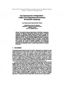
Hence the statement “It is snowing” has meaning in itself, regardless of the context, and the valuation will depend on the particular context, which is called a possible world , a self-consistent state of affairs. For Kripke, a possible world is the real, existing world, apart from the fact that certain aspects have been explicitly changed. A possible world therefore becomes the context of application of expressions. There are a wide variety of intensional logics, which encompass problems pertaining to time, belief, situation, etc. We are most interested here in those logics where the possible contexts of evaluation can be viewed as points in a multidimensional space [50], hence the term multidimensional logic. For example, temporal logic define expressions that vary in a time dimension, which are valuated at different instants. This means that each expression has possibly a different value, depending on the instant in which it is evaluated. Basically, intensional logics add dimensions to logical expressions, and non-intensional logics can be viewed as “constant” in all possible dimensions. Intensional operators are defined to navigate in the dimensions enabled by a particular intensional logic. For example, in temporal logics, we have operators such as before and after that enable us to navigate in time. Of course, for navigation to occur, we must have some dimension tags to hold on to. So in every dimension defined on a given intensional logic, we have a set of tags, along with a partial order defined on the latter. These dimension tags, along with the dimension names they belong to, are used to define the current context of evaluation of the expressions. For example, we can have an expression E: E: the average temperature for this month here is greater than 0 ◦ C.

The truth value of this expression depends on the context in which it is evaluated. The two intensional operators in this expression are this month and here, which refer respectively to the time and space dimension, which itself is generally viewed as being three-dimensional. Let us “freeze” the space context to the city of Quebec. Figure 2.1 gives the yearly temperature at this space context, for an entire year (data freely estimated by the author). The time dimension tags are the months of the year. So along the time dimension, we have the following valuation for the above expression, with T and F respectively standing for true and false: E

=

Ja F

Fe Mr Ap Ma Jn Jl F F F T T T

Au Se Oc No T T F F

De F

We can see with the latter valuation notation that expression E actually varies in the time dimension. Constructing from our Earth-bound view of time and space, we can elaborate multidimensional expressions such as:


8

30 20 10 0 -10 -20 Ja Fe Mr Ap Ma Jn Jl Au Se Oc No De

Figure 2.1: Approximate yearly temperature in Quebec E 0 : the temperature above here is greater than 0◦ C.

Given the altitude dimension tags {0, 5000, 10000, . . .}, we have a valuation for E 0 :

E0

=

0 5 10 >15

km km km km

Ja F F F F

Fe F F F F

Mr F F F F

Ap F F F F

Ma T F F F

Jn T T F F

Jl T T T F

Au T T F F

Se T F F F

Oc F F F F

No F F F F

De F F F F

We see here that each line of the valuation can be interpreted by itself as “frozen” in space. Thus, using intensional (context-switching) operators, we can navigate in the valuation: E 00 : the temperature at 10000 m is greater than 0◦ C. E 00

=

Ja F

Fe F

Mr F

Ap F

Ma F

Jn F

Jl T

Au F

Se F

Oc F

No F

De F

The latter “at” navigation operator is not indexical; it does not depend on the context of evaluation. We can also have relative intensional operators, as in the following indexical expression: E 000 : the temperature 5000 m above here and 6 months ago was greater than 0 ◦ C.

The latter sentence has the following valuation:

E 000 =

0m 5 km 10 km >15 km

Ja T T F F

Fe T F F F

Ma F F F F

Ap F F F F

Ma F F F F

Jn F F F F

Jl F F F F

Au F F F F

Se F F F F

Oc F F F F

No F F F F

De T F F F


9

It is precisely this concept of navigation through a context space that has been retained in intensional programming (as used by the Lucid language), which allows computations to be made according to the current context. To better illustrate possible worlds semantics, we can consider the World Wide Web, where the URLs are the possible worlds. Each link on the Web can be understood as a context-switching operator, and the browser even provides the user with contextswitching operators in the back and forward buttons. However, the Web and the different browsers have not been designed on an intensional basis. This is simply an intensional view of the Web. Intensional programming takes these ideas and goes one step further. A systematic set of operators, called intensional operators, is required to allow general navigation in any given context. For example, on Web pages, one can go to any other page, but there are few relative context-switching operators, apart from the back and forward buttons, which are only for navigation in the very specific “time” dimension of a single query session. Depending on the domain, operators might be of the form up, down, right, left, back and forward; north, east, south and west; or yesterday, today and tomorrow. However, more general operators would enable navigation along a number of dimensions. An intensional programming language retains therefore two aspects from intensional logic. First, at the syntactic level, are context-switching operators, called intensional operators. Second, at the semantic level, is the use of possible worlds semantics (in conjunction, of course, with other semantic notions, such as least fixpoints and closures).

2.2

Lucid: from program verification to intensions Hindsight is always 20/20 But looking back, it’s still a bit fuzzy —Dave Mustaine (1996)

The Lucid language is an intensional programming language whose intensional properties were historically refined through successive generalizations. We begin here by a brief history of the evolution of the language. Then, as an introduction to the language, we give some typical example programs taken from the two main references on Lucid, [4, 69]. For more details on the syntax and semantics of the language, the reader is referred to the following chapter.


2.2.1

10

Pipeline dataflows

The origins of Lucid date back to 1974. At that time, Ashcroft and Wadge were working on a purely declarative language in which iterative algorithms could be expressed naturally [6]. Their work fits into the broad area of research into program semantics and verification. It would turn out, serendipitously, that their work would also be relevant to the dataflow networks and coroutines of Kahn and MacQueen [43, 44]. In the original Lucid (whose operators are underlined in the following text), streams were defined in a pipeline manner, with two separate definitions: one for the initial element, and another one for the subsequent elements. For example, the equations first X = 0 next X = X + 1 define variable X to be a stream, such that x0 = 0 xi+1 = xi + 1 In other words, X = (x0 , x1 , . . . , xi , . . .) = (0, 1, . . . , i, . . .) Similarly, the equations first X = X next Y = Y + next X define variable Y to be the running sum of X, i.e. y0 = x 0 yi+1 = yi + xi+1 In other words, Y = (y0 , y1 , . . . , yi , . . .) =

µ

i(i + 1) 0, 1, . . . , ,... 2

¶


11

It soon became clear that a new operator fby (followed by) could be used to define the typical situation. Hence the above two variables could be defined as follows: X = 0 fby X + 1 Y = X fby Y + next X Hence, we can summarize the three basic operators of the original Lucid. Definition 1 If X = (x0 , x1 , . . . , xi , . . .) and Y = (y0 , y1 , . . . , yi , . . .), then (1) first X (2) next X (3) X fby Y

def

= (x0 , x0 , . . . , x0 , . . .) = (x1 , x2 , . . . , xi+1 , . . .) def = (x0 , y0 , y1 , . . . , yi−1 , . . .) def

Clearly, analogues can be made to list operations, where first corresponds to hd, next corresponds to tl, and fby corresponds to cons. When these operators are combined with Landin’s ISWIM [47] (If You See What I Mean), essentially typed λ-calculus with syntactic sugar, it becomes possible to define complete Lucid programs. The following three derived operators have turned out to be very useful (we will use them later in the text): Definition 2 (1) X wvr Y (2) X asa Y (3) X upon Y

def

= if first Y then X fby (next X wvr next Y ) else (next X wvr next Y ) def = first (X wvr Y ) def = X fby (if first Y then (next X upon next Y ) else ( X upon next Y ))

Where wvr stands for whenever, asa stands for as soon as and upon stands for advances upon.

2.2.2

Tagged-token dataflows

With the original Lucid operators, one could only define programs with pipeline dataflows, i.e. in which the (i + 1)-th element in a stream is only computed once the i-th element has


12

been computed. This situation is potentially wasteful of resources, since the i-th element might not necessarily be required. More importantly, it only allows sequential access into streams. By taking a different approach, it is possible to have random access into streams, using an index # corresponding to the current position. No longer are we manipulating infinite extensions (streams), rather we are defining computation according to a context (here a single integer). We have set out on the road to intensional programming. Everything is now redefined in terms of the operators # and @. In terms of the three original operators, these are defined as: Definition 3 (1) #

def

(2) X @ Y

def

= 0 fby (# + 1) = if Y = 0 then first X else (next X) @ (Y − 1)

Below, we will give definitions for the original operators using these two new operators. In so doing, we will use the following axioms. Axiom 1 Let i ≥ 0. (1) (2) (3) (4) (5) (6) (7) (8) (9)

[c]i = c [X + c]i = [X]i + c [first X]i = [X]0 [next X]i = [X]i+1 [X fby Y ]0 = [X]0 [X fby Y ]i+1 = [Y ]i if true then [X]i else [Y ]i = [X]i if false then [X]i else [Y ]i = [Y ]i [if C then X else Y ]i = if [C]i then [X]i else [Y ]i

Before we give the new definitions of the standard Lucid operators, we show some basic properties of @ and #. We will use throughout the discussion here [X]i instead of xi , as it allows for greater readibility. Furthermore, we will, as is standard, write X = Y whenever we have (∀i : i ≥ 0 : [X]i = [Y ]i )


13

Proposition 1 Let i ≥ 0. (1) [#]i = i (2) [X @ Y ]i = [X][Y ]i Proof (1) Proof by induction over i. Base step (i = 0). [#]0 = [0 fby (# + 1)]0 = [0]0 = 0

Defn. 3.1 Axiom 1.5 Axiom 1.1

Induction step (i = k + 1). Suppose (∀i : i ≤ k : [#]i = i). [#]k+1 = = = =

[0 fby (# + 1)]k+1 [# + 1]k [#]k + 1 k+1

Defn. 3.1 Axiom 1.6 Axiom 1.2 Ind. Hyp.

Hence (∀i : i ≥ 0 : [#]i = i). (2) Let i ≥ 0. We will prove by induction over yi that yi ≥ 0 ⇒ [X @ Y ]i = [X][Y ]i . Base step (yi = 0). [X @ Y ]i = = = = = =

[if Y = 0 then first X else (next X) @ (Y − 1)]i if [Y = 0]i then [first X]i else [(next X) @ (Y − 1)]i if [Y ]i = 0 then [first X]i else [(next X) @ (Y − 1)]i [first X]i [X]0 [X][Y ]i

Defn. 3.2 Axiom 1.9 Axiom 1.2 Axiom 1.7 Axiom 1.3 Hypothesis

Induction step (yi = k + 1). Suppose (∀i : i ≤ k : [#]i = i). [X @ Y ]i = = = = = = = =

[if Y = 0 then first X else (next X) @ (Y − 1)]i if [Y = 0]i then [first X]i else [(next X) @ (Y − 1)]i if [Y ]i = 0 then [first X]i else [(next X) @ (Y − 1)]i [(next X) @ (Y − 1)]i [next X][Y −1]i [next X][Y ]i −1 [X][Y ]i −1+1 [X][Y ]i

Hence (∀i : i ≥ 0 : [Y ]i ≥ 0 ⇒ ([X @ Y ]i = [X][Y ]i )).

Defn. 3.2 Axiom 1.9 Axiom 1.2 Axiom 1.8 Ind. Hyp. Axiom 1.2 Axiom 1.4 Arith. 2


14

Definition 4 (1) (2) (3) (4)

def

first X next X X fby Y X wvr Y

= = def = def =

X@0 X @ (# + 1) if # = 0 then X else Y @ (# − 1) X@T where T = U fby U @ (T + 1) U = if Y then # else next U end def = first (X wvr Y ) def = X@W where W = 0 fby if Y then (W + 1) else W end def

(4.1) (4.2) (5) (6)

X asa Y X upon Y

(6.1)

The advantage of these new definitions is that they do not use any form of recursive function definitions. Rather, all of the definitions are iterative, and in practice, more easily implemented in an efficient manner. We prove below that the new definitions are equivalent to the (underlined) old ones. Proposition 2 first X = first X.

Proof Let i ≥ 0. Then [first X]i = = = =

[X @ 0]i [X][0]i [X]0 [first X]i

Hence first X = first X. Proposition 3 next X = next X.

Defn. 4.1 Prop. 1.2 Axiom 1.1 Axiom 1.3 2


15

Proof Let i ≥ 0. Then [next X]i = = = = =

[X @ (# + 1)]i [X][#+1]i [X][#]i +1 [X]i+1 [next X]i

Hence next X = next X.

Defn. 4.2 Prop. 1.2 Axiom 1.2 Prop. 1.1 Axiom 1.4 2

Proposition 4 X fby Y = X fby Y .

Proof Proof by induction over i. Base step (i = 0). [X fby Y ]0 = = = = = =

[if # = 0 then X else Y @ (# − 1)]0 if [# = 0]0 then [X]0 else [Y @ (# − 1)]0 if [#]0 = 0 then [X]0 else [Y @ (# − 1)]0 if 0 = 0 then [X]0 else [Y @ (# − 1)]0 [X]0 [X fby Y ]0

Defn. 4.3 Axiom 1.9 Defn. 1.2 Prop. 1.1 Axiom 1.7 Axiom 1.5

Induction step (i = k + 1). [X fby Y ]k+1 = = = = = = = = =

[if # = 0 then X else Y @ (# − 1)]k+1 if [# = 0]k+1 then [X]k+1 else [Y @ (# − 1)]k+1 if [#]k+1 = 0 then [X]k+1 else [Y @ (# − 1)]k+1 if k + 1 = 0 then [X]k+1 else [Y @ (# − 1)]k+1 [Y @ (# − 1)]k+1 [Y ][#−1]k+1 [Y ][#]k+1 −1 [Y ]k [X fby Y ]k+1

Hence (∀i : i ≥ 0 : [X fby Y ]i = [X fby Y ]i ). Hence fby = fby .

Defn. 4.3 Axiom 1.9 Axiom 1.1 Prop. 1.1 Axiom 1.8 Prop. 1.2 Axiom 1.2 Prop. 1.1 Axiom 1.6 2

The proof for wvr is more complicated, as it requires relating an iterative definition to a recursive definition. We will therefore need four lemmas that refer to variables T and U in the text in Definitions 4.4.1 and 4.4.2. In addition, we must define the rank of a Boolean stream. Finally, we will have to introduce another set of axioms, that allow us to compare two entire streams, as opposed to particular elements in the two streams.


16

Axiom 2 Let i ≥ 0. (1) (2) (3) (4) (5) (6) (7) (8)

X0 = X [X i ]0 = [X]i first X i = [X]i next X i = X i+1 next (X fby Y ) = Y (first X) fby Y = X fby Y if true then X else Y = X if false then X else Y = Y

Definition 5 Let Y be a Boolean stream. def

(1) rank(−1, Y ) = −1 def (2) rank(i + 1, Y ) = min{k : k > rank(i, Y ) : [Y ]k = true} Below, we write ri for rank(i, Y ).

Lemma 1 (∀i : i ≥ −1 : (∀j : ri < j ≤ ri+1 : X j wvr Y j = X ri+1 wvr Y ri+1 )).

Proof Let i ≥ −1. Proof by downwards induction over j. Note that ri < ri+1 . Base step (j = ri+1 ). X ri+1 wvr Y ri+1 = X ri+1 wvr Y ri+1

Identity

Induction step (j = k − 1, j > ri ). X k−1 wvr Y k−1 = if first Y k−1 then X k−1 fby X k wvr Y k else X k wvr Y k = if [Y ]k−1 then X k−1 fby X k wvr Y k else X k wvr Y k = X k wvr Y k = X ri+1 wvr Y ri+1 Hence, (∀i : i ≥ −1 : (∀j : ri < j ≤ ri+1 : X j wvr Y j = X ri+1 wvr Y ri+1 )). Lemma 2 (∀i : i ≥ 0 : (X wvr Y )i = X ri wvr Y ri ).

Defn. 2.1 Axiom 2.3 Axiom 2.8 Ind. Hyp. 2


17

Proof Proof by induction over i. Base step (i = 0). (X wvr Y )0 = X wvr Y = X 0 wvr Y 0 = X r0 wvr Y r0

Axiom 2.1 Axiom 2.1 Lemma 1

Induction step (i = k + 1). (X wvr Y )k+1 = next ((X wvr Y )k ) = next (X rk wvr Y rk ) = next (if first Y rk then X rk fby X rk +1 wvr Y rk +1 else X rk +1 wvr Y rk +1 ) = next (if [Y ]rk then X rk fby X rk +1 wvr Y rk +1 else X rk +1 wvr Y rk +1 ) rk = next (X fby X rk +1 wvr Y rk +1 ) = X rk +1 wvr Y rk +1 = X rk+1 wvr Y rk+1

Axiom 2.4 Ind. Hyp. Defn. 2.1 Axiom 2.3 Axiom 2.7 Axiom 2.5 Lemma 1

Hence, (∀i : i ≥ 0 : (X wvr Y )i = X ri wvr Y ri ).

2

Lemma 3 (∀i : i ≥ −1 : (∀j : ri < j ≤ ri+1 : [U ]j = ri+1 )).

Proof Let i ≥ −1. Proof by downwards induction over j. Note that ri < ri+1 . Base step (j = ri+1 ). [U ]ri+1 = = = =

[if Y then # else next U ]ri+1 if [Y ]ri+1 then [#]ri+1 else [next U ]ri+1 [#]ri+1 ri+1

Defn. 4.4.2 Axiom 1.9 Axiom 1.7 Prop. 1.1

Induction step (j = k − 1, j > ri ). [U ]k−1 = = = = =

[if Y then # else next U ]k−1 if [Y ]k−1 then [#]k−1 else [next U ]k−1 [next U ]k−1 [U ]k ri+1

Hence, (∀i : i ≥ −1 : (∀j : ri−1 < j < ri : [U ]j = ri+1 )).

Defn. 4.4.2 Axiom 1.9 Axiom 1.8 Axiom 1.4 Ind. Hyp. 2


18

Lemma 4 (∀i : i ≥ 0 : [T ]i = ri ).

Proof Proof by induction over i. Base step (i = 0). [T ]0 = [U fby U @ (T + 1)]0 = [U ]0 = r0

Defn. 4.4.1 Axiom 1.5 Lemma 3

Induction step (i = k + 1). [T ]k+1 = = = = = =

[U fby U @ (T + 1)]k+1 [U @ (T + 1)]k [U ][T +1]k [U ][T ]k +1 [U ]rk +1 rk+1

Hence, (∀i : i ≥ 0 : [T ]i = ri ).

Defn. 4.4.1 Axiom 1.6 Prop. 1.2 Axiom 1.2 Ind. Hyp. Lemma 3 2

Proposition 5 X wvr Y = X wvr Y .

Proof [X wvr Y ]i = = = = = = = = = =

[X @ T ]i [X][T ]i [X]ri [X ri ]0 [X ri fby X ri +1 wvr Y ri +1 ]0 [if [Y ]ri then X ri fby X ri +1 wvr Y ri +1 else X ri +1 wvr Y ri +1 ]0 [if first Y ri then X ri fby X ri +1 wvr Y ri +1 else X ri +1 wvr Y ri +1 ]0 [X ri wvr Y ri ]0 [(X wvr Y )i ]0 [X wvr Y ]i

Hence X wvr Y = X wvr Y . Proposition 6 X asa Y = X asa Y .

Defn. 4.4 Prop. 1.2 Lemma 4 Axiom 1.2 Axiom 1.6 Axiom 2.7 Axiom 2.3 Defn. 2.1 Lemma 2 Axiom 2.2 2


19

Proof X asa Y

= = = =

first (X wvr Y ) first (X wvr Y ) first (X wvr Y ) X asa Y

Hence X asa Y = X asa Y .

Defn. 4.5 Prop. 5 Prop. 2 Defn. 2.2 2

Lemma 5 (∀i : i ≥ 0 : (X upon Y )i = X [W ]i upon Y i )

Proof Proof by induction over i. Base step (i = 0). (X upon Y )0 = = = =

X upon Y X 0 upon Y 0 X [0 fby ...]0 upon Y 0 X [W ]0 upon Y 0

Axiom 2.1 Axiom 2.1 Defn. 2.3 Defn. 4.6.1

Induction step (i = k + 1). (X upon Y )k+1 = next ((X upon Y )k ) = next (X [W ]k upon Y k ) = if (first Y k ) then (X [W ]k +1 upon Y k+1 ) else (X [W ]k upon Y k+1 ) = if [Y ]k then (X [W ]k+1 upon Y k+1 ) else (X [W ]k upon Y k+1 ) = (X (if [Y ]k then [W ]k+1 else [W ]k ) ) upon Y k+1 = X [W ]k+1 upon Y k+1 Hence, (∀i : i ≥ 0 : (X upon Y )i = X [W ]i upon Y i ) Proposition 7 X upon Y = X upon Y .

Axiom 2.4 Ind. Hyp. Defn. 2.3 and Axiom 2.5 Axiom 2.4 Defn. 4.6.1 Substit. Defn. 4.6.1 2


20

Proof Let i ≥ 0. Then [X upon Y ]i = = = = = =

[X @ W ]i [X][W ]i [X [W ]i ]0 [X [W ]i fby . . .]0 [X [W ]i upon Y i ]0 [X upon Y ]i

Hence X upon Y = X upon Y .

Defn. 4.6 Prop. 1.2 Axiom 2.2 Axiom 1.5 Defn. 2.3 Lemma 5 2

Now that the new definitions are shown to be equivalent, we can generalize and head off in the negative direction as well: Definition 6 (1) prev X (2) X fby Y

def

= X @ (# − 1) = if # ≤ 0 then X else Y @ (# − 1)

def

With the increased power of this new version of Lucid came the first attempts at implementation. First tries involved the coroutine/dataflow approaches used at the time for the implementation of dataflow languages [43, 44]. However, since stream elements were no longer necessarily computed in order, these approaches failed. Cargill, May and Gardin then independently came up with implementations directly based on the formal semantics of Lucid. Ostrum finally extended the technique and came up with the Luthid interpreter [53], which was the direct precursor of the pLucid interpreter, the first widelydistributed implementation of Lucid. See reference [69] for a full discussion. The implementation technique used by these interpreters, called eduction, is still used in the latest implementation of Lucid, namely the GLU compiler (see Chapter 4). Eduction can be described as “tagged-token demand-driven dataflow”, in which data elements (tokens) are computed on demand following a dataflow network defined in Lucid. Data elements flow in the normal flow direction (from producer to consumer) and demands flow in the reverse order, both being tagged with their current context of evaluation.

2.2.3

Multidimensional dataflows

Lucid as presented up to now allows one to define simple streams, but it does not allow any sort of subcomputation, in which the subcomputation itself requires streams. To do


21

this requires a new dimension. Initially, this was done in Lucid by freezing values, using an operator called is current [69]. Unfortunately the semantics was unwieldy. A more general solution was provided in IndexicalLucid [28]. Subcomputations could take place in arbitrary dimensions, and all indexical operators would be parametrized by one or several dimensions. The # and @ operators became #.d and @.d, where #.d allows one to query about part of the evaluation context, rather than the entire evaluation context. Similarly, @.d allows one to change part of the evaluation context, which might be highly dimensional. The basic operators thus become: first.d X next.d X prev.d X X fby.d Y X wvr.d Y

= = = = =

X @.d 0; X @.d (#.d+1); X @.d (#.d-1); if #.d {{X0,X1,Q},{X1,Xnew,Q}}

int(X0) + int(Xnew)); * (X1_d-X0_d)/(Xnew_d-X0_d);

CHAPTER 6. TENSORLUCID: INTENSIONAL SCIENTIFIC PROGRAMMING 105

cross(S1,S2) inter.d(X,S) sqnorm(S) sq(S) dnext.d(S) dprev.d(S) prevnext.d(S) avg.d(S) avgnext.d(S) addup.d(S) unfold(f,X) unfold2(f,X,F) end;

= = = = = = = = = = = =

(S1_r)*(S2_l) - (S1_l)*(S2_r); S + frac(X_d) * dnext.d S; sq(S_l) + sq(S_m) + sq(S_r); S*S; next.d S - S; S - prev.d S; prev.d S + next.d S; 0.5 * (S + prev.d S); 0.5 * (S + next.d S); 0.5 * S + 0.25 * (prevnext.d S); f.x(f.y(f.z(X)); f.x(X,f.y(X,f.z(X,F)));

The example given in this section shows that is it quite possible to take an existing Fortran program, to study and analyze it and then to produce an equivalent Lucid program that is much much shorter and clearer and in which parallelism is much greater. We have also shown that our intensional tensor syntax simplifies the creation of Lucid programs starting from differential equations.

6.3.2

Relativistic particle displacement

The latter example used simple vectors, i.e. rank-one tensors and in the quite simple case of orthogonal linear tridimensional manifold. To really show the possibilities of TensorLucid we present here an example using higher-ranking tensors in a Boyer–Linquist manifold, a quadridimensional spherical orthogonal manifold. This example is inspired from a C program written by Blackburn [10]. The problem consists in computing the trajectory of particles in the vicinity of a black hole. The extreme gravitational field generated by the black hole implies the presence of relativistic effects on the trajectories of particles approaching it, as pointed out by Einstein in his general theory of relativity [18]. This problem is sufficiently complex to present the fundamental concepts of higherranking tensors, but is simple enough to be explained and programmed in few lines. The system of equations is defined in the Boyer–Linquist coordinate system B : (t, r, θ, φ). The black hole has mass M , moment J and rotates in direction φ. The

CHAPTER 6. TENSORLUCID: INTENSIONAL SCIENTIFIC PROGRAMMING 106 metric tensor gij has the form:  gtt 0 0 gφt  0 grr 0 0     0 0 gθθ 0  gtφ 0 0 gφφ 

with, at every point (t, r, θ, φ) : gtt = −(1 − (2M r/Σ))

gφt = −(2aM r sin2 (θ/Σ))

gtφ = gφt

grr = Σ/∆ gθθ = Σ gφφ = r2 + a2 + 2M ra2 sin2 (θ) sin2 (θ/Σ) a = J/M ∆ = r2 − 2M r + a2 Σ = r2 + a2 cos2 (θ)

The corresponding TensorLucid program follows those definitions in a quite straight forward manner. First, the definition of the manifold dimensions is: manifold BoyerLinquist(t,r,theta,phi); Then, the function kerr_metric defines the metric in every possible component of the tensor: kerr_metric(p) = g_i_j where g = 0; g_t_t = -(1 - (2 * M * r/Sigma)); g_phi_t = -(2 * a * M * r * sq(sin(theta/Sigma)); g_t_phi = g_phi_t; g_r_r = Sigma/Delta; g_theta_theta = Sigma; g_phi_phi = sq(r) + sq(a) + 2 * M * r * sq(a) * sq(sin(theta)) * sq(sin(theta/Sigma));

CHAPTER 6. TENSORLUCID: INTENSIONAL SCIENTIFIC PROGRAMMING 107 a Delta Sigma r theta sq(x) end;

= = = = = =

J/M; sq(r) - 2*M*r + sq(a); sq(r) + sq(a) * sq(cos(theta)); p^r; p^theta; x * x;

where g=0 defines the default value for the undefined components in the where clause. The problem here is to compute the acceleration ai of a particle having initial speed ui at point pi . The system of equations to calculate this is the following: ¡ i ¢ ai = − Γjk ∗ uj ∗ uk

i Γjk

g il (glj,k + glk,j − gkj,l ) = 2

where gij,k =

∂gij ∂xk

In TensorLucid, we cannot (yet) automatically do the algebraic transformations, so the different forms of g must be named differently: kerr_geodesic(p,u) = a where aî = -(Gammaî_j_k*u^j*u^k); Gammaî_j_k = g2î^l*(g3_l_j,,k+g3_l_k,,j-g3_k_j,,l)/2; g1_i_j = kerr_metric(p^l); g2î^j = inverse(g1_i_j); g3_i_j,,k = kerr_metric(p^l+(k*delta)) - g1_i_j; end;

6.4

Summary

The objective of TensorLucid was to allow one to write computer programs that closely correspond, at both the syntactic and semantic levels, to the original equations. The two examples given in this chapter, particle-in-cell 3-D simulation of plasmas and relativistic

CHAPTER 6. TENSORLUCID: INTENSIONAL SCIENTIFIC PROGRAMMING 108 particle displacement, have shown that this goal has been achieved. All this was done simply by introducing syntactic extensions to PartialLucid. GLU represents the only Lucid compiler available at the moment. Unfortunately, GLU does not enable the dimensions and functions as first-class values, which is one of the key principles used in TensorLucid. This prevents us from testing the Lucid programs presented in this Chapter. However, we plan to design an entirely new version of intensional programming environment. The guidelines for this project are presented in Chapter 8.

Chapter 7 Conclusion When I am working on a problem, I never think about beauty. I only think about the problem. But when I am finished, if the solution is not beautiful, I know it is wrong. —Buckminster Fuller(1895-1983)

7.1

Introduction

Scientific programming has been, and continues to be, one of the driving forces of Computer Science. Since their invention in the 1940s, computers have been ever-present in the resolution of calculation-intensive scientific problems. Some computers have been designed specifically for the resolution of scientific problems, and many programming languages have been designed to enable the simulation of these problems. Parallel computers and high-speed networks are more and more readily available and more scientists turn now more naturally to computer simulations for experimentation and validation of their theories. However, the dazzling evolution of hardware is not followed by a corresponding evolution in scientific programming software systems. Scientific programming should be doable by people of the scientific community, without having to learn about obscure features such as state, store and cache. Unfortunately, to this day, reality is quite different. Most languages now used for high-performance scientific programming are parallel versions of imperative programming languages used since the early days of scientific programming, such as Fortran or C. As it was pointed out in Chapter 1, these languages have proven to be inappropriate for the natural expression of problems involving scientific equations and programming in these languages requires an extensive Computer Science — read arcane — knowledge from the programmer. 109

CHAPTER 7. CONCLUSION

110

This chapter presents existing programming and translation systems used in the scientific programming community, as well as a comparison of the latter with the intensional programming approach to scientific computing.

7.2

Scientific programming requirements

In order to make a comparison between the standard (extensional) and intensional approaches to scientific computing, we first introduce the requirements of scientific programming languages and environments. (1) Natural expression of scientific equations. The language should be able to express differential and tensor equations in a form as close as possible to the original equations. This involves the natural expression of metadimensional — or dimensionally abstract — concepts, which are intensional by nature. (2) Intrinsic notion of multidimensional continuum. Scientific equations define the behavior of forces and fluids in a multidimensional continuum. These dimensions naturally represent the usual space dimensions, but can also include other dimensions such as time, temperature, density, pressure, etc. The integration of dimensions as part of the basic building blocks of the language should be a crucial part of the design of a scientific programming language. (3) Minimize Computer Science knowledge requirements. The language and programming environment should enable members of the scientific community to develop scientific programs on their own, with a limited knowledge of concepts not specific to the subject under study. (4) High-speed execution. Most scientific programs are complex enough to need high-performance hardware for efficient execution. Thus, scientific programming languages should enable the parallel execution of programs.

7.3

Extensional approach to scientific programming

There are currently two major approaches to scientific programming. The first, mathematical programming languages, are mostly used for small-scale simulations. Such languages generally offer symbolic programming and user-friendly programming environments. The


111

second, parallel programming languages, are used in most large-scale simulations, as the need for efficiency outweighs all other aspects.

7.3.1

Mathematical programming systems

Mathematical programming language and systems offer the possibility to naturally express and compute sets of mathematical equations through symbolic programming. Maple, Mathematica and Matlab are among the most complete and widely used mathematical programming systems. However, these systems take the general approach of having a separate, ad hoc, approach for each kind of mathematical notation. This is true, for example, for the tensor calculus, which is implemented as a package in Maple. The intensional approach to the tensor calculus allowed tensors to be naturally expressed, simply as syntactic sugar, by supposing an underlying multidimensional continuum that is consistent with physical reality. With respect to performance, all these systems generally rely on interpretation to generate an executable version of the equations. Since these systems can run on generalpurpose shared-memory multiprocessor (SMP) machines, performance can be very good. Furthermore, most of these systems provide facilities to compile computation-intensive parts of the program to achieve better performance. However, the generated code cannot be finetuned to achieve outstanding results on the most powerful parallel machines.

7.3.2

Parallel programming languages and environments

One of the main concerns in scientific programming is the high-speed execution of the generated programs. In most cases, the fastest execution possible can be achieved using parallel processing architectures. To harness such computing power is normally not an easy task, as many issues, such as the arrangement of the memory hierarchy and of inter-processor communication, are non-trivial. In many cases, the synchronization and communication processes involved in parallel processing have to be managed explicitly by the programmer. Some parallel programming languages, such as GLU or other dataflowbased programming languages, provide facilities that enable the implicit representation of parallelism in programs. However, most of the programming languages conventionally used by scientists, namely Fortran and C / C++, were not designed to naturally or implicitly express the concurrency and communication aspects of parallel programming. Some efforts have been made towards the parallelization of these languages. These set out into two main methods of parallelization, namely data parallelism and task parallelism.


112

Data and task parallelism Data parallelism supposes large data elements on which computations are to be performed homogeneously over the entire data area. Data-parallel languages provide constructions to automatically segment and communicate the parallelized data on the processors involved. This method is obviously extensional and is thus limited in terms of meta-dimensional expressiveness. However, a great number of sequential scientific programs can very easily parallelized using data-parallelism, which makes this method very attractive for the parallelization of simple programs. Examples of data-parallel version of mainstream scientific programming languages include: Fortran D [25], HPF [29] and pC++ [34]. Task parallelism supposes computation-intensive problems where the exploitable parallelism does not lie in the distribution of data, but in the distribution of the program code itself. Task-parallel languages either provide constructs to explicitly specify the parallelism in the program, or provide a precompiler using dataflow analysis to extract the parallelism in sequential programs. Task-parallel version of mainstream scientific programming languages include: CC++ [15], Fortran M [30], Cilk [36]. This kind of parallelism is not restricted to an extensional view of computation. It lends itself more naturally for the expression of the intensional concepts present in scientific programming. GLU can be viewed as a task-parallel version of C relying on a dataflow program skeleton. Other languages or programming environments aim at the incorporation of data- and task-parallelism. This interesting increase in generality obviously raises the level of complexity of such systems. These generally rely on a mix of explicit constructs and compiletime program analysis to generate parallel programs. Examples include: PARADIGM [7], HPC++ [33] and Ada95 [64], Dataflow oriented parallel programming environments In the early 70’s, Kahn and MacQueen [43, 44] invented dataflow graphs, which turned out to become a very simple and powerful tool for the representation of parallel programs. The nodes of a dataflow graph can be viewed as functions that accept the input data from its input arcs and place their output on its output arcs. Parallelism lies in the fact that each independent input arc of a node can be computed in parallel. Following this concept, several parallel computation systems have been designed. HeNCE [8] and CODE [11] are two highly related graphical parallel programming environments based on dataflow graphs. In both of these, one associates with each node a function (the computation element) along with a firing rule and a routing rule that can be used to simulate demand-driven computation. Thus, the model used by these two


113

programming environments would be worth more exploration if we are to look into the possiblility to design an enhanced intensional programming system (see Chapter 8). One of the major problems of these systems is that scientific programs are more naturally written as a set of equations than a dataflow graph. As discussed in Chapter 4, the parallel programming environment GLU is also based on dataflow graphs. However, rather than representing it graphically, the graph is programmed in a textual form using Lucid. It has been stated (page 38) that there exists an injective correspondence between a dataflow graph and a Lucid program. So we could design a compiler that would translate Lucid programs into dataflow graphs (and inversely) to get the best of both worlds: a convenient graphical interface and a textual representation highly related to the original equations of the problem. Other noteworthy examples of parallel programming environments include Phred [9], Schedule [19], ALEX [24], Paragraph [23], Paralex [26], VERDI [35], PPSE [49], D 2 R [60], Poker [63], PFG [65] and Neptune[68].

7.4

Intensional approach

Scientific programming is about the manipulation of multidimensional objects (or concepts) evolving in a multidimensional continuum. We have shown that tensors are intensional, multidimensional and even meta-dimensional (see Sections 6.1 and 6.1). The mainstream scientific programming languages can manipulate multidimensional objects, but in the general case these manipulations are extensional. Each object has a fixed number of dimensions, and the dimensions most often do not have names (e.g. array declarations in Fortran or C). Each dimension must be referred to explicitly, even if it is not part of the computation. It is not possible to define meta-dimensional (i.e. dimensionally abstract) statements, operations or functions other than with an extensional method. Intensional programming is about defining objects in a multidimensional context. The introduction of dimensions as first-class values in TensorLucid enables full-fledge metadimensional manipulations of multidimensional objects. Using these new features of Lucid, we have shown in Chapter 6 that there typically exists a one-to-one correspondence between the mathematical specification of a scientific problem and a TensorLucid program. Furthermore, GLU has proven that it is possible to compile Lucid programs towards parallel executables yielding outstanding overall performance [1, 2, 42, 37, 38, 39]. Future versions of GLU will be designed in an intensional manner, where the multidimensional


114

nature of the problems will be used to guide the distribution of the problems through the memory hierarchies and to the various processors. These two demonstrations allow us to pave the way to a new vision of scientific programming in which mathematical specifications can be directly programmed in a natural way, and the operational simulations can run on high-end parallel computers or clusters of workstations for exceptional performances. Unfortunately, we cannot readily prove this by operational results. In the course of this thesis, we made some generalizations to the Lucid language, which are not yet implemented in the GLU compiler. It is now up to us to design a whole new version of intensional programming environment that will enable us to prove the possibilities of TensorLucid. In this projected software system, the compiler will find its theoretical foundations in the semantic specifications given in Chapter 3 and the discussion of Chapter 4. The operational details of the implementation of the run-time system will be mostly inspired by the GLU system, with several updates taken from the experience we aquired in the course of this thesis.

7.5

Summary

Scientific programming is certainly one of the key fields in the future of Computer Science. Up to now, no programming system provides the scientific community with a tool fully complying with the requirements given above. Therefore, it is now up to us to find a solution to this problem by combining our new intensional approach to scientific programming with the practical experience acquired by the scientific community up to now. However, to be widely recognized as a possible solution, intensional programming needs more visibility. As it will be pointed out in Chapter 8, intensional programming can also be used to resolve other critical problems in Computer Science, including software versioning, multidimensional spreadsheets and reactive programming. The best way to attract the attention of computer scientists is to achieve a breakthrough result using an elegant and natural solution. We feel that the development of a general and efficient intensional programming tool would enable the intensional programming community to prove that intensional programming can be used to naturally and efficiently solve several of the most demanding problems of Computer Science.

Chapter 8 Future Work My interest is in the future because I am going to spend the rest of my life there. —Charles F. Kettering (1896-1958) This chapter presents future work which will be the direct consequence of the research undertaken in the course of this thesis.

8.1

General intensional programming system

Intensional programming has been successfully applied to topics as diverse as reactive programming, software configuration, scientific programming and Web page design. However, these projects have all been developed in isolation. GLU is the most general intensional programming tool presently available. However, experience has proven that, while being very efficient, the GLU [40] system is not flexible (see Chapter 5). Given that the Lucid [4, 69] language is evolving continually, there is an important need for the successor to GLU to be able to stand the heat of evolution. As a result, we propose to provide a set of flexible and general tools for the intensional programmer. We propose the design and implementation of a General Eduction Engine (GEE) based on a General Intensional Programming Language (GIPL). The language should be capable of expressing all extensions to Lucid, as well as other intensional languages for software configuration, reactive programming, spreadsheets, etc., proposed to this day. The GEE should be designed in a modular manner to permit the eventual replacement of each of its components—at compile-time or even at run-time—to improve the efficiency of specific components. 115

CHAPTER 8. FUTURE WORK

116

The latter two will be the two main components of the general intensional programming system (GIPS), which aims to provide a high-performance intensional programming system usable for the programmation of any problems of intensional nature. The main outcome of the proposed research is to show that the intensional approach to computing can be applied systematically to the building of efficient software.

General intensional programming language (GIPL) The GIPL must be general enough for existing (functional) intensional programming language to be translated into it. This means that the following features must be included: • dimensions and function identifiers must be first-class values; • different kinds of dimensions should be allowed: – discrete dimensions of arbitrary types (integers, integer lists, etc.); – ordered dimensions (total orders, partial orders); – space dimensions (for vectors and tensors); • tags should not just designate individual points, but entire regions; • encapsulation must be provided; • default definitions must be provided.

Specific intensional programming languages (SIPL) As the GIPL is being developed, the existing intensional programming formalisms will be translated into the GIPL. These include: • intensional versioning (Plaice and Wadge [57]); • intensional attribute grammars (Tao and Wadge); • intensional spreadsheets (Du and Wadge [21]); • intensional scientific programming (Paquet and Plaice); • intensional reactive programming (Gagné and Plaice [31]).


117

Of course, nothing will prevent us from combining these different approaches. For example, interactive scientific programming, combining version control and scientific programming, is of great interest: While a parallel program is running, the code can be changed on the fly, and only those intermediate results that are affected need be recomputed. Similarly, using the intensional attribute grammars to build the successive versions of the GIPL would be of great merit.

General eduction engine (GEE) The eduction engine is the core of the implementation of the GIPS. It provides a way of generating and managing demands and a warehouse to store values of demands previously computed. The General Eduction Engine will be based on the experience acuired with GLU (see Chapter 5). Demand generator The eduction engine generates demands according to the dataflow graph defined in the Lucid part of the program. For each demand, the eduction engine checks in the eduction warehouse if a value has already been calculated. If so, the value is fetched from the warehouse and no computation occurs. If the demand requires computation, the result can be calculated either locally or on a remote computing unit. Remote computations will be first implemented using IPC, though, as is the case for all components of the system, efforts will be made towards sufficient modularity to enable further plug-in of other remote procedure call schemes. As soon as a demand is made, it is placed in a demand queue, to be removed only when the demand has been successfully computed. This way of doing has been successfully implemented in GLU and provides a highly fault-tolerant system to the users. The eventual fault of a remote computing unit will simply trigger a reissuing of the faulty demand. Since many parallel programs require long execution times, fault tolerance is of prime importance; it comes free with the demand-driven model of computation. Also as most parallel and/or distributed software are enhanced versions of sequential ones, we will enable the system to reuse existing code by permitting demands to take the form of sequential threads. This also permits to bypass one of the greatest limitations of demand-driven computation, namely the communication overhead imposed by finegrained remote computation. The use of sequential threads as computation grains has been successfully implemented in GLU. However, one of the weaknesses of GLU is that demands can only be requested for a single cell at a time. If a single operation has to be made on an entire region of the value space, communication overhead is inefficiently multiplied by the number of cells in the region.


118

Eduction warehouse The second part of the eduction engine is the eduction warehouse, which is strongly related to Web caches and proxies. The eduction engine uses the dataflow’s context tags to build a store of values that already have been computed (the eduction warehouse). One of the key concerns when using caches is the use of a garbage collecting algorithm adapted to the current situation. The use of a garbage collector configured or adapted to the current situation is of prime importance to obtain high performance. Again, the use of highly modular programming and a multi-level specification of software interfaces will enable the system to accept other garbage collecting algorithms with minimal programming cost. Different eductive techniques Eduction can be a simple one-time process, as in computing in Lucid, or a two-stage show, as in spreadsheet calculations. There are, in fact, myriads of forms of eduction. For example, some kinds of version selection correspond more to an aggregation process than to a selection process: All versions that correspond to the version description are chosen, and these are all coalesced into a single version. This process, for example, was taken by m.c. schraefel, in her Ph.D. thesis [62]. As a result, the design of the GEE must allow for different eductive techniques to be defined very easily, and that finetuning be made sufficiently easy that efficient implementation be possible.

8.2

Summary

While having been a great breakthrough in parallel/distributed and intensional computing in the mid 90’s, the GLU project has since been put on the ice by SRI because of the departure of its main developers, namely Jagannathan and Dodd. This situation has to be remedied, considering the number of interesting applications of intensional programming. Specifically, we think that the scientific programming community could greatly benefit from the development of an enhanced version of GLU following the guidelines we gave in Chapter 4. The natural expression of scientific equations has not been proved to be accessible to any high-performance programming system. We also consider that the software crisis is mainly due to the explosion of the size of software systems. In this context, software versioning systems become of prime importance. Again, we feel that intensional programming could be the solution to the problem, providing a natural way of specifying software versioning specifications.


119

The development of a highly modular and configurable high-performance intensional programming system should provide a general tool for the resolution of many problems in these critical years of Computer Science.

Appendix A Fortran Code for Tristan

C C C C

program tf2(tty,tape59=tty,output,disperr=output, 1tf2out,tape3=tf2out,tf2in,tape2=tf2in, 2tekout,tape9=tekout) TRIdimensional STANford code, TRISTAN, fully electromagnetic, with full relativistic particle dynamics. Written during spring 1990 by OSCAR BUNEMAN, with help from TORSTEN NEUBERT and KEN NISHIKAWA. common /partls/x(8192),y(8192),z(8192),u(8192),v(8192),w(8192) common /fields/ex1(8192),ey1(8192),ez1(8192),bx1(8192), &by1(8192),bz1(8137) &,sm(27),q,qe,qi,qme,qmi,rs,ps,os,c &,ms(27),mx,my,mz,ix,iy,iz,lot,maxptl,ions,lecs,nstep real me,mi dimension label(10) dimension t(128)

C The sizes of the particle and field arrays must be chosen in C accordance with the requirements of the problem and the limitation C of the computer memory. The choice ’8192’ (with the bz1 array C curtailed to accommodate the remainder of the fields common) was C made to suit the segmented memory of a PC. Any changes in these C array sizes must be copied exactly into the COMMON statements of C the "surface", "mover" and "depsit" subroutines. C Fields can be treated as single-indexed or triple-indexed: C For CRAY-s, the first two field dimensions should be ODD, as here: dimension ex(21,19,20),ey(21,19,20),ez(21,19,20), &bx(21,19,20),by(21,19,20),bz(21,19,20) equivalence(ex1(1),ex(1,1,1)),(ey1(1),ey(1,1,1)),(ez1(1),ez(1, &1,1)),(bx1(1),bx(1,1,1)),(by1(1),by(1,1,1)),(bz1(1),bz(1,1,1)) c

120

APPENDIX A. FORTRAN CODE FOR TRISTAN label(1)=8htf2001 label(2)=8htf2002 label(3)=8htf2003 label(4)=8htf2004 label(5)=8htf2005 label(6)=8htf2006

C

C

C C C C C C C C

C C C C

maxptl=8192 mx=21 my=19 mz=20 Strides for single-indexed field arrays: ix=1 iy=mx iz=iy*my lot=iz*mz Miscellaneuos constants: qe=-.0625 qi=.0625 me=.0625 mi=1. qme=qe/me qmi=qi/mi c=.5 Our finite difference equations imply delta_t = delta_x = delta_y = delta_z = 1. So c must satisfy the Courant condition. The bx,by and bz arrays are really records of c*Bx, c*By, c*Bz: this makes for e b symmetry in Maxwell’s equations. Otherwise, units are such that epsilon_0 is 1.0 and hence mu_0 is 1/c**2. This means that for one electron per cell (see example of particle initialisation below) omega_p-squared is qe**2/me. For use in the boundary field calculation: rs=(1.-c)/(1.+c) tsq=.1666667 ps=(1.-tsq)*c/(1.+c) os=.5*(1.+tsq)*c/(1.+c) Data for smoothing: the currents fed into Maxwell’s equations are smoothed by convolving with the sequence .25, .5, .25 in each dimension. Generate the 27 weights ("sm") and index displacements ("ms"): n=1 do 1 nz=-1,1 do 1 ny=-1,1 do 1 nx=-1,1 sm(n)=.015625*(2-nx*nx)*(2-ny*ny)*(2-nz*nz) ms(n)=ix*nx+iy*ny+iz*nz 1 n=n+1

121

APPENDIX A. FORTRAN CODE FOR TRISTAN C C C C C C C C C C

C

C C C C

C C

In the particle arrays the ions are at the bottom, the electrons are stacked against the top, the total number not exceeding maxptl: The number of ions, "ions", need not be the same as the number of electrons, "lecs". The code treats unpaired electrons as having been initially dissociated from infinitely heavy ions which remain in situ. Initialise the particles: Place electrons in same locations as ions for zero initial net charge density. Keep particles 2 units away from the lower boundaries of the field domain, 3 units away from the upper boundaries. For instance, fill the interior uniformly: ions=0 do 80 k=1,mz-5 do 80 j=1,my-5 do 80 i=1,mx-5 ions=ions+1 x(ions)= 2.5+i y(ions)= 2.5+j 80 z(ions)= 2.5+k Put electrons in the same places: lecs=ions do 4 n=1,lecs x(n+maxptl-lecs)=x(n) y(n+maxptl-lecs)=y(n) 4 z(n+maxptl-lecs)=z(n) Initialise velocities: these should not exceed c in magnitude! For thermal distributions, add three or four random numbers for each component and scale. Initialise random number generator: lk=12345 lp=29 do 85 n=1,ions u(n)=0.046875*(rndm(lk,lp)+rndm(lk,lp)+rndm(lk,lp)) v(n)=0.046875*(rndm(lk,lp)+rndm(lk,lp)+rndm(lk,lp)) w(n)=0.046875*(rndm(lk,lp)+rndm(lk,lp)+rndm(lk,lp)) u(maxptl-lecs+n)=0.1875*(rndm(lk,lp)+rndm(lk,lp)+rndm(lk,lp)) v(maxptl-lecs+n)=0.1875*(rndm(lk,lp)+rndm(lk,lp)+rndm(lk,lp)) 85 w(maxptl-lecs+n)=0.1875*(rndm(lk,lp)+rndm(lk,lp)+rndm(lk,lp)) Initialise the fields, typically to uniform components, such as just a uniform magnetic field parallel to the z-axis: do 5 k=1,mz do 5 j=1,my do 5 i=1,mx ex(i,j,k)=0. ey(i,j,k)=0. ez(i,j,k)=0. bx(i,j,k)=0. by(i,j,k)=0.

122

APPENDIX A. FORTRAN CODE FOR TRISTAN

C C C C C C

C C

C C C C C C C C C C C C C C C C C C C C C C C C C

5 bz(i,j,k)=c*1.5 (Remember that bx,by,bz are really c*Bx, c*By, c*Bz.) Initial fields, both electric and magnetic, must be divergence-free. Part of the Earth’s magnetic field would be ok. If the Earth is included in the field domain, its magnetic dipole field is readily established by maintaining a steady ring current in the Earth’s core. Begin time stepping last=2 nstep=1 Before moving particles, the magnetic field is Maxwell-advanced by half a timestep: 6 do 7 i=1,mx-1 do 7 j=1,my-1 do 7 k=1,mz-1 bx(i,j,k)=bx(i,j,k) + (.5*c) * & (ey(i,j,k+1)-ey(i,j,k)-ez(i,j+1,k)+ez(i,j,k)) by(i,j,k)=by(i,j,k) + (.5*c) * & (ez(i+1,j,k)-ez(i,j,k)-ex(i,j,k+1)+ex(i,j,k)) 7 bz(i,j,k)=bz(i,j,k) + (.5*c) * & (ex(i,j+1,k)-ex(i,j,k)-ey(i+1,j,k)+ey(i,j,k)) Now move ions: call mover(1,ions,qmi) and electrons: call mover(maxptl-lecs+1,maxptl,qme) The Maxwell-advance of the fields begins with another half-step advance of the magnetic field since for Maxwell’s equations the B - information and the E - information must be staggered in time. In space, their information is also staggered. Here we show the locations where field components are recorded:

z ^ | | | *---------------Ey---------------* /| | / | | / | | Ex | | / | | / | | / | | * | | | | |

123

APPENDIX A. FORTRAN CODE FOR TRISTAN C | | | C | | | C | Ez Bx Ez C | | | C | | | C | | | C | By | | C | | | C | | | C | | | C Ez | | C | | | C | | | C | | | C | *---------------Ey---------------*-----> y C | / / C | / / C | / / C | Ex Bz Ex C | / / C | / / C |/ / C *---------------Ey---------------* C / C / C / C x C C C Ex(i,j,k) = value of Ex at x=i+.5, y=j, z=k C Ey(i,j,k) = value of Ey at x=i, y=j+.5, z=k C Ez(i,j,k) = value of Ez at x=i, y=j, z=k+.5 C C Bx(i,j,k) = value of Bx at x=i, y=j+.5, z=k+.5 C By(i,j,k) = value of By at x=i+.5, y=j, z=k+.5 C Bz(i,j,k) = value of Bz at x=i+.5, y=j+.5, z=k C C Maxwell’s laws are implemented (to central difference C accuracy) in the form: C C Change of flux of B through a cell face C = - circulation of E around that face C C Change of flux of E through a cell face of the offset grid C = circulation of B around that face - current through it C C Second half-advance of magnetic field:

124


C C

C

C C

C C C C C C C C C C C C

do 8 i=1,mx-1 do 8 j=1,my-1 do 8 k=1,mz-1 bx(i,j,k)=bx(i,j,k) + (.5*c) * & (ey(i,j,k+1)-ey(i,j,k)-ez(i,j+1,k)+ez(i,j,k)) by(i,j,k)=by(i,j,k) + (.5*c) * & (ez(i+1,j,k)-ez(i,j,k)-ex(i,j,k+1)+ex(i,j,k)) 8 bz(i,j,k)=bz(i,j,k) + (.5*c) * & (ex(i,j+1,k)-ex(i,j,k)-ey(i+1,j,k)+ey(i,j,k)) Front,right and top layers of B must be obtained from a special boundary routine based on Lindman’s method: call surface(by,bz,bx,ey,ez,ex,iy,iz,ix,my,mz,mx,1) call surface(bz,bx,by,ez,ex,ey,iz,ix,iy,mz,mx,my,1) call surface(bx,by,bz,ex,ey,ez,ix,iy,iz,mx,my,mz,1) call edge(bx,ix,iy,iz,mx,my,mz,1) call edge(by,iy,iz,ix,my,mz,mx,1) call edge(bz,iz,ix,iy,mz,mx,my,1) Full advance of the electric field: do 9 i=2,mx do 9 j=2,my do 9 k=2,mz ex(i,j,k)=ex(i,j,k) + c * & (by(i,j,k-1)-by(i,j,k)-bz(i,j-1,k)+bz(i,j,k)) ey(i,j,k)=ey(i,j,k) + c * & (bz(i-1,j,k)-bz(i,j,k)-bx(i,j,k-1)+bx(i,j,k)) 9 ez(i,j,k)=ez(i,j,k) + c * & (bx(i,j-1,k)-bx(i,j,k)-by(i-1,j,k)+by(i,j,k)) Boundary values of the E - field must be provided at rear, left and bottom faces of the field domain: call surface(ey,ez,ex,by,bz,bx,-iy,-iz,-ix,my,mz,mx,lot) call surface(ez,ex,ey,bz,bx,by,-iz,-ix,-iy,mz,mx,my,lot) call surface(ex,ey,ez,bx,by,bz,-ix,-iy,-iz,mx,my,mz,lot) call edge(ex,-ix,-iy,-iz,mx,my,mz,lot) call edge(ey,-iy,-iz,-ix,my,mz,mx,lot) call edge(ez,-iz,-ix,-iy,mz,mx,my,lot) The currents due to the movement of each charge q are applied to the E-M fields as decrements of E-flux through cell faces. The movement of particles which themselves cross cell boundaries has to be split into several separate moves, each only within one cell. Each of these moves contributes to flux across twelve faces. Ions and electrons are processed in two loops, changing the sign of the charge in-between. These loops cannot be vectorised: particles get processed one by one. Here is a good place to insert the statements for applying boundary conditions to the particles, such as reflection, periodicity, replacement by inward moving thermal or streaming particles, etc. Split and deposit ions currents:

125

APPENDIX A. FORTRAN CODE FOR TRISTAN q=qi n1=1 n2=ions 52 do 53 n=n1,n2 C Previous position: x0=x(n)-u(n) y0=y(n)-v(n) z0=z(n)-w(n) C Reflect particles at x=3, x=mx-2, y=3, y=my-2, z=3, z=mz-2: u(n)=u(n)*sign(1.,x(n)-3.)*sign(1.,mx-2.-x(n)) x(n)=mx-2.- abs(mx-5.-abs(x(n)-3.)) v(n)=v(n)*sign(1.,y(n)-3.)*sign(1.,my-2.-y(n)) y(n)=my-2.- abs(my-5.-abs(y(n)-3.)) w(n)=w(n)*sign(1.,z(n)-3.)*sign(1.,mz-2.-z(n)) z(n)=mz-2.- abs(mz-5.-abs(z(n)-3.)) C Alternatively, apply periodicity to particles: CC x(n)=x(n)+sign(.5*(mx-5.),mx-2.-x(n))-sign(.5*(mx-5.),x(n)-3.) CC y(n)=y(n)+sign(.5*(my-5.),my-2.-y(n))-sign(.5*(my-5.),y(n)-3.) CC z(n)=z(n)+sign(.5*(mz-5.),mz-2.-z(n))-sign(.5*(mz-5.),z(n)-3.) 53 call xsplit(x(n),y(n),z(n),x0,y0,z0) C The split routines call the deposit routine. if(n2.eq.maxptl)go to 54 C Split and deposit electron currents: q=qe n1=maxptl-lecs+1 n2=maxptl go to 52 C Countdown: 54 nstep=nstep+1 c write out x,y,z positions of selected particles npick=n/100 ntsf=npick/6 do 40 iw=1,ntsf ii1=(iw-1)*6+1 ii2=ii1+5 40 write(9,100) (x(itt),itt=ii1,ii2),label(1) write(9,101) label(1) do 41 iw=1,ntsf ii1=(iw-1)*6+1 ii2=ii1+5 41 write(9,100) (y(itt),itt=ii1,ii2),label(1) write(9,101) label(1) do 42 iw=1,ntsf ii1=(iw-1)*6+1 ii2=ii1+5 42 write(9,100) (z(itt),itt=ii1,ii2),label(1)

126


100 101

write(9,101) label(1) format(6(1pe12.5),a8) format(72x,a8)

c

C C C C c

if (nstep.le.last) go to 6 The user must decide what information is to be written out at each timestep, what only occasionally, and what only at the end. It may be wise to write out both COMMONS before stopping: they can then be read in again for a continuation of the run.

call exit(1) end C -------subroutine surface(bx,by,bz,ex,ey,ez,ix,iy,iz,mx,my,mz,m00) C (Field components are treated as single-indexed in this subroutine) dimension bx(1),by(1),bz(1),ex(1),ey(1),ez(1) common /fields/ex1(8192),ey1(8192),ez1(8192),bx1(8192), &by1(8192),bz1(8137) &,sm(27),q,qe,qi,qme,qmi,rs,ps,os,c &,ms(38) m0=m00+iz*(mz-1) assign 5 to next 6 m=m0 do 2 j=1,my-1 n=m do 1 i=1,mx-1 bz(n)=bz(n)+.5*c*(ex(n+iy)-ex(n)-ey(n+ix)+ey(n)) 1 n=n+ix 2 m=m+iy go to next (5,7) 7 return 5 m=m0+ix+iy do 4 j=2,my-1 n=m C Directive specifically for the CRAY cft77 compiler: cdir$ ivdep do 3 i=2,mx-1 bx(n)=bx(n-iz)+rs*(bx(n)-bx(n-iz))+ps*(bz(n)-bz(n-ix))-os*( &ez(n+iy)-ez(n))-(os-c)*(ez(n+iy-iz)-ez(n-iz))-c*(ey(n)-ey(n-iz)) by(n)=by(n-iz)+rs*(by(n)-by(n-iz))+ps*(bz(n)-bz(n-iy))+os*( &ez(n+ix)-ez(n))+(os-c)*(ez(n+ix-iz)-ez(n-iz))+c*(ex(n)-ex(n-iz)) 3 n=n+ix 4 m=m+iy assign 7 to next go to 6 end

127

APPENDIX A. FORTRAN CODE FOR TRISTAN C

-----------subroutine edge(bx,ix,iy,iz,mx,my,mz,m00) dimension bx(1) lx=ix*(mx-1) ly=iy*(my-1) lz=iz*(mz-1) n=m00+iy+lz cdir$ ivdep do 1 j=2,my-1 bx(n)=bx(n+ix)+bx(n-iz)-bx(n+ix-iz) bx(n+lx)=bx(n+lx-ix)+bx(n+lx-iz)-bx(n+lx-ix-iz) 1 n=n+iy n=m00+ly+iz cdir$ ivdep do 2 k=2,mz-1 bx(n)=bx(n+ix)+bx(n-iy)-bx(n+ix-iy) bx(n+lx)=bx(n+lx-ix)+bx(n+lx-iy)-bx(n+lx-ix-iy) 2 n=n+iz n=m00+ly+lz cdir$ ivdep do 3 i=1,mx bx(n)=bx(n-iy)+bx(n-iz)-bx(n-iy-iz) bx(n-ly)=bx(n-ly+iy)+bx(n-ly-iz)-bx(n-ly+iy-iz) bx(n-lz)=bx(n-lz-iy)+bx(n-lz+iz)-bx(n-lz-iy+iz) 3 n=n+ix return end C-------subroutine mover(n1,n2,qm) common /partls/ x(8192),y(8192),z(8192),u(8192),v(8192),w(8192) C (Field components are treated as single-indexed in this subroutine) common /fields/ ex(8192),ey(8192),ez(8192), &bx(8192),by(8192),bz(8137) &,sm(27),q,qe,qi,qme,qmi,rs,ps,os,c &,ms(27),mx,my,mz,ix,iy,iz,lot,maxptl,ions,lecs,nstep do 1 n=n1,n2 C Cell index & displacement in cell: i=x(n) dx=x(n)-i j=y(n) dy=y(n)-j k=z(n) dz=z(n)-k l=i+iy*(j-1)+iz*(k-1) C Field interpolations are tri-linear (linear in x times linear in y C times linear in z). This amounts to the 3-D generalisation of "area C weighting". A modification of the simple linear interpolation formula

128

APPENDIX A. FORTRAN CODE FOR TRISTAN C C C C C C C C C C

C

C

C C

C

f(i+dx) = f(i) + dx * (f(i+1)-f(i)) is needed since fields are recorded at half-integer locations in certain dimensions: see comments and illustration with the Maxwell part of this code. One then has first to interpolate from "midpoints" to "gridpoints" by averaging neighbors. Then one proceeds with normal interpolation. Combining these two steps leads to: f at location i+dx = half of f(i)+f(i-1) + dx*(f(i+1)-f(i-1)) where now f(i) means f at location i+1/2. The halving is absorbed in the final scaling. E-component interpolations: f=ex(l)+ex(l-ix)+dx*(ex(l+ix)-ex(l-ix)) f=f+dy*(ex(l+iy)+ex(l-ix+iy)+dx*(ex(l+ix+iy)-ex(l-ix+iy))-f) g=ex(l+iz)+ex(l-ix+iz)+dx*(ex(l+ix+iz)-ex(l-ix+iz)) g=g+dy* & (ex(l+iy+iz)+ex(l-ix+iy+iz)+dx*(ex(l+ix+iy+iz)-ex(l-ix+iy+iz))-g) ex0=(f+dz*(g-f))*(.25*qm) -----------f=ey(l)+ey(l-iy)+dy*(ey(l+iy)-ey(l-iy)) f=f+dz*(ey(l+iz)+ey(l-iy+iz)+dy*(ey(l+iy+iz)-ey(l-iy+iz))-f) g=ey(l+ix)+ey(l-iy+ix)+dy*(ey(l+iy+ix)-ey(l-iy+ix)) g=g+dz* & (ey(l+iz+ix)+ey(l-iy+iz+ix)+dy*(ey(l+iy+iz+ix)-ey(l-iy+iz+ix))-g) ey0=(f+dx*(g-f))*(.25*qm) -----------f=ez(l)+ez(l-iz)+dz*(ez(l+iz)-ez(l-iz)) f=f+dx*(ez(l+ix)+ez(l-iz+ix)+dz*(ez(l+iz+ix)-ez(l-iz+ix))-f) g=ez(l+iy)+ez(l-iz+iy)+dz*(ez(l+iz+iy)-ez(l-iz+iy)) g=g+dx* & (ez(l+ix+iy)+ez(l-iz+ix+iy)+dz*(ez(l+iz+ix+iy)-ez(l-iz+ix+iy))-g) ez0=(f+dy*(g-f))*(.25*qm) --------B-component interpolations: f=bx(l-iy)+bx(l-iy-iz)+dz*(bx(l-iy+iz)-bx(l-iy-iz)) f=bx(l)+bx(l-iz)+dz*(bx(l+iz)-bx(l-iz))+f+dy* & (bx(l+iy)+bx(l+iy-iz)+dz*(bx(l+iy+iz)-bx(l+iy-iz))-f) g=bx(l+ix-iy)+bx(l+ix-iy-iz)+dz*(bx(l+ix-iy+iz)-bx(l+ix-iy-iz)) g=bx(l+ix)+bx(l+ix-iz)+dz*(bx(l+ix+iz)-bx(l+ix-iz))+g+dy* & (bx(l+ix+iy)+bx(l+ix+iy-iz)+dz*(bx(l+ix+iy+iz)-bx(l+ix+iy-iz))-g) bx0=(f+dx*(g-f))*(.125*qm/c) -----------f=by(l-iz)+by(l-iz-ix)+dx*(by(l-iz+ix)-by(l-iz-ix)) f=by(l)+by(l-ix)+dx*(by(l+ix)-by(l-ix))+f+dz* & (by(l+iz)+by(l+iz-ix)+dx*(by(l+iz+ix)-by(l+iz-ix))-f) g=by(l+iy-iz)+by(l+iy-iz-ix)+dx*(by(l+iy-iz+ix)-by(l+iy-iz-ix)) g=by(l+iy)+by(l+iy-ix)+dx*(by(l+iy+ix)-by(l+iy-ix))+g+dz* & (by(l+iy+iz)+by(l+iy+iz-ix)+dx*(by(l+iy+iz+ix)-by(l+iy+iz-ix))-g) by0=(f+dy*(g-f))*(.125*qm/c)

129

APPENDIX A. FORTRAN CODE FOR TRISTAN C

C C

C

C

C

C

C

-----------f=bz(l-ix)+bz(l-ix-iy)+dy*(bz(l-ix+iy)-bz(l-ix-iy)) f=bz(l)+bz(l-iy)+dy*(bz(l+iy)-bz(l-iy))+f+dx* & (bz(l+ix)+bz(l+ix-iy)+dy*(bz(l+ix+iy)-bz(l+ix-iy))-f) g=bz(l+iz-ix)+bz(l+iz-ix-iy)+dy*(bz(l+iz-ix+iy)-bz(l+iz-ix-iy)) g=bz(l+iz)+bz(l+iz-iy)+dy*(bz(l+iz+iy)-bz(l+iz-iy))+g+dx* & (bz(l+iz+ix)+bz(l+iz+ix-iy)+dy*(bz(l+iz+ix+iy)-bz(l+iz+ix-iy))-g) bz0=(f+dz*(g-f))*(.125*qm/c) --------First half electric acceleration, with relativity’s gamma: g=c/sqrt(c**2-u(n)**2-v(n)**2-w(n)**2) u0=g*u(n)+ex0 v0=g*v(n)+ey0 w0=g*w(n)+ez0 First half magnetic rotation, with relativity’s gamma: g=c/sqrt(c**2+u0**2+v0**2+w0**2) bx0=g*bx0 by0=g*by0 bz0=g*bz0 f=2./(1.+bx0*bx0+by0*by0+bz0*bz0) u1=(u0+v0*bz0-w0*by0)*f v1=(v0+w0*bx0-u0*bz0)*f w1=(w0+u0*by0-v0*bx0)*f Second half mag. rot’n & el. acc’n: u0=u0+v1*bz0-w1*by0+ex0 v0=v0+w1*bx0-u1*bz0+ey0 w0=w0+u1*by0-v1*bx0+ez0 Relativity’s gamma: g=c/sqrt(c**2+u0**2+v0**2+w0**2) u(n)=g*u0 v(n)=g*v0 w(n)=g*w0 Position advance: x(n)=x(n)+u(n) y(n)=y(n)+v(n) 1 z(n)=z(n)+w(n) return end -------subroutine xsplit(x,y,z,x0,y0,z0) if(ifix(x).ne.ifix(x0))go to 1 call ysplit(x,y,z,x0,y0,z0) return 1 x1=.5*(1+ifix(x)+ifix(x0)) y1=y0+(y-y0)*((x1-x0)/(x-x0)) z1=z0+(z-z0)*((x1-x0)/(x-x0)) call ysplit(x,y,z,x1,y1,z1)

130


C

C

C C

C

C

C

call ysplit(x1,y1,z1,x0,y0,z0) return end -------subroutine ysplit(x,y,z,x0,y0,z0) if(ifix(y).ne.ifix(y0))go to 1 call zsplit(x,y,z,x0,y0,z0) return 1 y1=.5*(1+ifix(y)+ifix(y0)) z1=z0+(z-z0)*((y1-y0)/(y-y0)) x1=x0+(x-x0)*((y1-y0)/(y-y0)) call zsplit(x,y,z,x1,y1,z1) call zsplit(x1,y1,z1,x0,y0,z0) return end -------subroutine zsplit(x,y,z,x0,y0,z0) if(ifix(z).ne.ifix(z0))go to 1 call depsit(x,y,z,x0,y0,z0) return 1 z1=.5*(1+ifix(z)+ifix(z0)) x1=x0+(x-x0)*((z1-z0)/(z-z0)) y1=y0+(y-y0)*((z1-z0)/(z-z0)) call depsit(x,y,z,x1,y1,z1) call depsit(x1,y1,z1,x0,y0,z0) return end -------subroutine depsit(x,y,z,x0,y0,z0) (Field components are treated as single-indexed in this subroutine) common /fields/ex(8192),ey(8192),ez(8192),bx(8192), &by(8192),bz(8137) &,sm(27),q,qe,qi,qme,qmi,rs,ps,os,c &,ms(27),mx,my,mz,ix,iy,iz,lot,maxptl,ions,lecs,nstep cell indices of half-way point: i=.5*(x+x0) j=.5*(y+y0) k=.5*(z+z0) displacements in cell of half-way point: dx=.5*(x+x0) - i dy=.5*(y+y0) - j dz=.5*(z+z0) - k l=i+iy*(j-1)+iz*(k-1) current elements: qu=q*(x-x0) qv=q*(y-y0) qw=q*(z-z0)

131

APPENDIX A. FORTRAN CODE FOR TRISTAN delt=.08333333*qu*(y-y0)*(z-z0) C Directive specifically for the CRAY cft77 compiler: cdir$ ivdep C (This will make the compiler use the "gather-scatter" hardware.) C If one desires NO smoothing (risking the presence of alias-prone C high harmonics), one can replace the statement "do 1 n=1,27" by C n=14 C and boost the value of q by a factor 8. do 1 n=1,27 ex(ms(n)+l+iy+iz)=ex(ms(n)+l+iy+iz)-sm(n)*(qu*dy*dz+delt) ex(ms(n)+l+iz)=ex(ms(n)+l+iz)-sm(n)*(qu*(1.-dy)*dz-delt) ex(ms(n)+l+iy)=ex(ms(n)+l+iy)-sm(n)*(qu*dy*(1.-dz)-delt) ex(ms(n)+l)=ex(ms(n)+l)-sm(n)*(qu*(1.-dy)*(1.-dz)+delt) ey(ms(n)+l+iz+ix)=ey(ms(n)+l+iz+ix)-sm(n)*(qv*dz*dx+delt) ey(ms(n)+l+ix)=ey(ms(n)+l+ix)-sm(n)*(qv*(1.-dz)*dx-delt) ey(ms(n)+l+iz)=ey(ms(n)+l+iz)-sm(n)*(qv*dz*(1.-dx)-delt) ey(ms(n)+l)=ey(ms(n)+l)-sm(n)*(qv*(1.-dz)*(1.-dx)+delt) ez(ms(n)+l+ix+iy)=ez(ms(n)+l+ix+iy)-sm(n)*(qw*dx*dy+delt) ez(ms(n)+l+iy)=ez(ms(n)+l+iy)-sm(n)*(qw*(1.-dx)*dy-delt) ez(ms(n)+l+ix)=ez(ms(n)+l+ix)-sm(n)*(qw*dx*(1.-dy)-delt) 1 ez(ms(n)+l)=ez(ms(n)+l)-sm(n)*(qw*(1.-dx)*(1.-dy)+delt) return end C ------------C Generator of randoms uniformily distributed between -.5 and .5 : function rndm(lucky,leap) C On CRAY-s, the next 5 statements should be replaced by: 1 lucky=and((lucky*261),32767) - and((lucky*261),32768) leap=leap-1 if(leap.ne.0)go to 2 leap=37 go to 1 2 rndm=(1./65536.)*float(lucky) return end

132

Bibliography [1] I. Agi. GLU for multidimensional signal processing. In Intensional Programming I, pages 135–148, Singapore, 1996. World Scientific. [2] I. Agi and R. Jagannathan. A portable fault-tolerant parallel software MPEG-1 encoder. In Multimedia: Tools and Applications, Kluwer Academic Press, Dordrecht, The Netherlands, 1996. [3] E. A. Ashcroft. Ferds—massive parallelism in Lucid. In Proceedings of the 1985 Phoenix Computer and Communications Conference, pages 16–21. IEEE, March 1985. [4] E. A. Ashcroft, A. A. Faustini, R. Jagannathan, and W. W. Wadge. Multidimensional, Declarative Programming. Oxford University Press, London, 1995. [5] E. A. Ashcroft and W. W Wadge. Lucid—A formal system for writing and proving programs. SIAM Journal on Computing, pages 336–354, September 1976. [6] E. A. Ashcroft and W. W Wadge. Lucid, a nonprocedural language with iteration. Communications of the ACM, pages 519–526, July 1977. [7] P. Banerjee, J. A. Chandy, M. Gupta, E. W. Hodges, J. G. Holm, A. Lain, D. J. Palermo, S. Ramaswamy, and E. Su. The PARADIGM Compiler for DistributedMemory Multicomputers. IEEE Computer, 28(10):37–47, October 1995. [8] Beguelin, Dongarra, Geist, Manchek, Moore, Newton, and Sunderam. HeNCE: A user’s guide. Technical report, Computer Science Department, University of Tennessee—Knoxville, 1994. [9] A. Beguelin and G. Nutt. Collected papers on PHRED. Technical Report CU-CS511-91, Department of Computer Science, University of Colorado, 1991. [10] J. K. Blackburn. GRPP, a scientific programming language preprocessor designed using lex and yacc. Computers in Physics, 8(1):98–112, 1994. 133

BIBLIOGRAPHY

134

[11] J. C. Browne. Visual programming and debugging for parallel computing. Technical Report TR94-229, Department of Computer Sciences, University of Texas at Austin, 1994. [12] O. Buneman. tristan: the 3-D E-M particle code. Unpublished manuscript. [13] O. Buneman, T. Neubert, and K. I. Nishikawa. Solar wind magnetosphere interaction as simulated by a 3-D EM particle code. IEEE Transactions on Plasma Science, 20(6):810–816, 1992. [14] R. Carnap. Meaning and Necessity. University of Chicago Press, 1989. second edition. [15] K. M. Chandy and C. Kesselman. CC++: A declarative concurrent object-oriented programming notation. Technical report, California Institute of Technology, March 1993. [16] D.L. Collins, C.J. Holmes, T.M. Peters, and A.C. Evans. Automatic 3-D model-based neuroanatomical segmentation. Human Brain Mapping, 3:190–208, 1995. [17] E. W. Dijkstra. A Discipline of Programming. Prentice-Hall, Englewood Cliffs, NewJersey, 1976. [18] P. A. M. Dirac. General Theory of Relativity. Princeton Landmarks in Physics. Princeton University Press, Princeton, New Jersey, 1996. [19] J. J. Dongarra and D. C. Sorenson. SCHEDULE: Tools for developing and analyzing parallel Fortran programs. Technical Report 86, Argonne National Laboratory MSCD, Chicago, 1986. [20] D. Dowty, R. Wall, and S. Peters. Introduction to Montague Semantics. D. Reidel, Dordrecht, The Netherlands, 1981. [21] W. Du and W. W. Wadge. A 3D spreadsheet based on intensional logic. IEEE Software, 1(7):78–89, 1990. [22] J. A. Eisele and R. M. Mason. Applied Matrix and Tensor Analysis. John Wiley and Sons, Inc., 1970. [23] D. A. Bailey et al. ParaGraph: Graph editor support for parallel programming environments. International Journal for Parallel Programming, April 1991. [24] D. Kozen et al. Visual Languages and Applications, chapter ALEX—An Alexical Programming Language. Plenum Press, New York, 1990.

BIBLIOGRAPHY

135

[25] G. C. Fox et al. The Fortran D language specification. Technical Report CRPCTR90079, Computer Science department, Rice University, 1990. ¨ Babaoglu et al. Paralex: An environment for parallel programming in distributed [26] O. systems. In Proceedings of the ACM International Conference on Supercomputing, July 1992. [27] A. A. Faustini. The equivalence of a denotational and an operational semantics of pure dataflow. PhD thesis, University of Warwick, Computer Science Department, Coventry, United Kingdom, 1982. [28] A. A. Faustini and R. Jagannathan. Indexical Lucid. In Proceedings of the Fourth International Symposium on Languages for Intensional Programming, Menlo Park, California, 1991. [29] High Performance Fortran Forum. High Performance Fortran Language Specification, version 2.0, January 1997. [30] I. Foster and K. M. Chandy. Fortran M: A language for modular parallel programming. Journal of Parallel and Distributed Computing, 25(1), February 1995. [31] J. R. Gagné. Time processing model. PhD thesis, Department of Computer Science, Laval University, Sainte-Foy, Canada, 1999. [32] D. Gallin. Intensional and Higher-Order Modal Logic: With Applications to Montague Semantics. North-Holland, Amsterdam, The Netherlands, 1975. [33] D. Gannon, P. Beckman, E. Johnson, T. Green, and M. Levine. HPC++ and the HPC++lib toolkit. Technical report, Department of Computer Science, Indiana University, 1997. [34] D. Gannon, S. Y. Yang, and P. Beckman. User guide for a portable C++ programming system, pC++. Technical report, Department of Computer Science, Indiana University, Bloomington, Indiana, U.S.A., 1994. [35] M. Graf. Principles of Visual Programming Systems, chapter Building a Visual Designer’s Environment. Prentice Hall, Englewood Cliffs, New-Jersey, 1990. [36] Supercomputing Technologies Group. Cilk 5.2 Reference Manual. MIT Laboratory for Computer Science, January 1998.

BIBLIOGRAPHY

136

[37] R. Jagannathan. Application experience with an implicitly parallel composition language. In Proceedings USENIX Very High Level Languages Symposium (VHLL94), Santa Fe, NM, 1994. [38] R. Jagannathan. Coarse-grain dataflow programming of conventional parallel computers. In J. L. Gaudiot G. Gao, L. Bic, editor, Advanced Topics in Dataflow Computing and Multithreading. IEEE Computer Society, April 1995. [39] R. Jagannathan. Toward a scalably efficient parallel implementation of a hybrid intensional language. In Proceedings of International Conference on High Performance Computing, New Delhi, December 1995. Tata McGraw Hill. [40] R. Jagannathan and C. Dodd. GLU programmer’s guide. Technical report, SRI International, Menlo Park, California, 1996. [41] R. Jagannathan and C. Dodd. Implementing glu on dynamic heterogeneous systems. In Proceedinngs of the 9th International Symposium on Languages for Intensional Programming, pages 19–25. Technical report, SRI International, Menlo Park, CA, 1996. [42] R. Jagannathan, C. Dodd, and I. Agi. GLU: A high-level system for granular dataparallel programming. Concurrency: Practice and Experience, (1):63–83, 1997. [43] G. Kahn. The semantics of a simple language for parallel processing. In Proceedings of the IFIP Congress ’74, pages 471–475, Amsterdam, 1974. Elsevier North-Holland. [44] G. Kahn and D. B. MacQueen. Coroutines and networks of parallel processes. In Proceedings of the IFIP Congress ’77, pages 993–998, Amsterdam, 1977. Elsevier North-Holland. [45] S. Kripke. Naming and Necessity. Harvard University Press, Cambridge, MA, 1980. [46] L. Lamport. LATEX, A Document Preparation System. User’s guide and Reference Manual. Addison-Wesley, 1994. [47] P. J. Landin. The next 700 programming languages. Communications of the ACM, 9(3):157–166, 1966. [48] T. Levi-Civita. Le problème des n corps en relativité générale. Number 116 in Mémorial des Sciences Mathématiques. Gauthier-Villars, Paris, France, 1950. [49] T. G. Lewis and W. Rudd. Architecture of the parallel programming support environment. In Proceedings of CompCon’90, San Fransisco, February 1990.

BIBLIOGRAPHY

137

[50] M. Marx and Y. Venema. Multidimensional Modal Logic. Kluwer Academic Publishers, Dordrecht, The Netherlands, 1997. [51] P. Neelin. MINC programmer’s guide. Technical report, Montreal Neurological Institute, Montreal, Canada, 1993. [52] P. Neelin. MINC programmer’s reference manual. Technical report, Montreal Neurological Institute, Montreal, Canada, 1993. [53] C. B. Ostrum. The Luthid 1.0 Manual. Department of Computer Science, University of Waterloo, Waterloo, Ontario, Canada, 1981. [54] A. L. Peratt. Physics of the Plasma Universe. Springer, New York, 1992. [55] J. Plaice. Particle in-cell simulation with Lucid. In E. A. Ashcroft, editor, Proceedings of the Seventh ISLIP, pages 53–56, SRI International, Menlo Park, California, 1994. [56] J. Plaice. Particle in-cell simulation with Lucid. In Intensional Programming I, pages 149–161. World Scientific, Singapore, 1995. [57] J. Plaice and W. W. Wadge. A new approach to version control. IEEE Transactions on Software Engineering, 3(19):268–276, 1993. [58] G. D. Plotkin. A Structural Approach to Operational Semantics. Computer Science Department, Aarhus University, Denmark, 1981. [59] G. Davis R. Rew and S. Emmerson. NetCDF’s user guide. Technical report, University corporation for atmosheric research, Boulder, Colorado, 1993. [60] J. Rost. D2 R: A dynamic dataflow representation for task scheduling. ACM SIGPLAN, 28(8), August 1993. [61] J. I. Sakai, T. Fushiki, and K. I. Nishikawa. A model of solar flares triggered by interactions between force-free current loops and plasmoids. Solar Physics, 158(301), 1995. [62] m.c. schraefel. Talking to Antigone. PhD thesis, Department of Computer Science, University of Victoria, Victoria, Canada, 1994. [63] L. Snyder. Poker 3.1: A programmer’s reference guide. Technical Report TR-85-0903, Department of Computer Science, University of Washington, Seattle, Washington, 1985.

BIBLIOGRAPHY

138

[64] M. J. Stift. Scientific programming with Ada 95: Object-oriented, parallel, and safe. Scientific Programming, 12(2):150–158, March/April 1998. [65] P. D. Stotts. Visual Languages and Visual Programming, chapter Graphical Operational Semantics for Visual Parallel Programming. Plenum Press, New York, 1990. [66] R. D. Tennent. Semantics of Programming Languages. Prentice Hall, Englewood Cliffs, New Jersey, 1991. [67] R. Thomason, editor. Formal Philosophy, Selected Papers of R. Montague. Yale University Press, New Haven, Connecticut, 1974. [68] B. Traversat. NEPTUNE: The Application of Coarse-Grain Dataflow Methods to Scientific Parallel Programming. PhD thesis, The Florida State University, 1990. [69] W. W. Wadge and E. A. Ashcroft. Lucid, the Dataflow Programming Language. Academic Press, London, 1985.

Index multidimensional, 6, 22, 26, 38, 40– 42 nodes, 38 pipeline, 6, 10, 11, 38 programming, 2, 5 tagged-token, 6, 20, 38 Debbabi, M., v definition environment (D), 43 demand-driven computation, 58, 117 Desharnais, J., v differential equations, 1, 2, 5, 94, 105 dimension as first class value, 21, 28, 29, 35 as first-class value, 36, 108, 113, 116 relevant, 40 Dodd, C., v, 56, 118

#, 12–15, 17, 20–22, 24, 43, 51, 53, 90 @, 12–15, 18, 20–22, 24, 43, 44, 51, 90 advances upon, 11 aggregates in TensorLucid, 92 Animal, 73–75, 77, 78, 80, 81 as soon as, 11 asa, 11, 14, 18, 19 Ashcroft, E. A., 5, 10 black hole, 105 Blackburn, J. K., 105 Buneman, O., 93 C, ii, iii, 1, 35, 37, 57–59, 65–71, 74, 80, 81, 105, 109, 111–113 CC++, 112 HPC++, 112 pC++, 112 Carnap, R., 6 Chaib-Drâa, B., v Christoffel symbol, 86 code reuse, 56, 57, 77, 117 computer simulation, 1, 109 context, 7–9, 12, 20, 21, 23 CRIM, v

eduction, 6, 20, 58 distributed, 60 garbage collection, 118 general eduction engine (GEE), 115, 117 semantics, 46 Einstein, A., 83 end of data, 37 engineering, 1, 84 eod, 30, 90 EPFL, v evaluation context (P), 44 extension, 6

dataflow, iii demand-driven, iii, 20 multidimensional, 6, 20, 40 network, 20, 24, 26–28, 32, 33, 57, 58, 112, 113

fault-tolerance, 117 139

140

INDEX Faustini, A. A., 38, 113 fby, 11–20, 53 first, 10–14, 16–19 followed by, 11 Fortran, ii, iii, 1, 35, 93, 105, 109, 111– 113, 120, 134, 135 Fortran D, 112 Fortran M, 112 HPF, 112 Fuller, B., 109 function as first class value, 22, 30 as first-class value, 108, 116 Gagné, J.-R., 53 generator, 58–60 GLU, ii, iii, v, 2, 3, 6, 20, 56–59, 65–73, 75, 77, 79–82, 108, 111–115, 117, 118, 133, 136 coding, 65 compilation, 70 debugging, 71, 79 global variables in programs, 66 hybrid nature of, 66 invocation from a C program, 69 load distribution, 67, 69 performance evaluation, 71 programming, 65 syntax, 57 C part, 58 Lucid part, 57 type definitions, 68 granularity, 56, 57, 66, 117 Hamming, 26 Hendrix, J. M., 73 Hipper, G., v if then else, 11–20

IndexicalLucid, 6, 21, 28 intension, 6 intensional, iii, 1, 2, 9 attribute grammars, 116 logic, iii, 5–7, 9 temporal logic, 7 programming, iii, 2, 3, 5, 9, 12, 22, 114, 115, 118 programming language GIPL, 115 SIPL, 116 programming language, GIPL, 116 programming system, GIPS, 116, 117 reactive programming, 116 scientific programming, 116 spreadsheets, 116 versioning, 116 iseod, 30, 37 ISWIM, 11, 21 Jagannathan, R., v, 56, 118 Kahn, G., 10, 38, 112 Kerr, 106 Kettering, C. .F., 115 Kripke, S., 6 Kropf, P. G., v Kuonen, P., v Landin, P. J., 11 load distribution, 57, 67 annotation (GLU), 69 Lorentz, 94, 98 Lucid, ii, iii, 2, 3, 5, 6, 9–12, 20–22, 26– 28, 31, 32, 35–41, 43–48, 50, 51, 53, 54, 56–58, 65, 66, 68, 69, 72, 79, 83–85, 88, 93, 96, 97, 99, 101, 105, 108, 113–115, 117, 118 semantics, 36, 43

141

INDEX rules (basic), 45 rules (with warehouse), 48 syntax, 36, 37 Luthid interpreter, 20 MacQueen, D. B., 10, 112 manifold, 84 Boyer–Linquist, 89, 105 declaration (TensorLucid), 89 Euclidian, 89 Marx, J. H., 83 Maxwell, J. C., 93 McGill University, 73 MNI, 73, 74 Montague, R., 6 multidimensional, 1, 2, 7, 21, 22, 35, 113 continuum, 110, 113 logic, 7 programming, 5 Mustaine, D., 9 navigation, 7–9, 22, 36 next, 10–17, 19 Ostrum, C., 20 parallel processing architecture, 57, 59 centralized generator (CGA), 59 semantics, 60 distributed generator (DGA), 60 dynamic (DDGA), 64 semantics, 61 static (SDGA), 62 generator-worker, 58 parallelization, 75, 111 data-parallelism, 112 task-parallelism, 112 ParAnimal, 73, 76–81 PartialLucid, 43, 50–52, 54, 88, 89, 91, 102, 103, 108

semantics, 50 rules, 52 syntax, 51 physics, 1, 5, 84 Plaice, J., v pLucid interpreter, 20 possible world, 7 prev, 20 programming environment parallel dataflow-based, 112 programming languages mathematical, 111 Maple, 111 Mathematica, 111 Matlab, 111 parallel, 111 Quebec, 8 query, 36 realign, 28 Reynolds, J. C., 36 ripe function executor (RFE), 59 RPC, 58 scientific programming, 1, 27, 35, 56, 109, 111, 114, 118 extensional approach, 110 intensional approach, 113 requirements, 110 semantics basis of Lucid’s, 5 operational, 43 possible worlds, 5, 9, 36 SGI, 79 software configuration, 115 Stanford University, 93 Strachey, C., 1

INDEX stream, 6, 10, 12, 20, 40 suspended function store (SFS), 58, 59 tensor, iii, 1, 2, 22, 83–87, 105, 111 as an intension, 87, 113 Boyer–Linquist, 91 coding in TensorLucid, 91 component, 84, 91 contravariant, 86 covariant, 86 declaration (TensorLucid), 91 Einstein, 85, 91 Euclidian, 91 field, 83, 88 TensorLucid, ii, iii, 2–4, 22, 36, 50, 54, 83, 87–93, 97, 102, 105–108, 113, 114 syntax, 88, 89 translation rules, 90 Tristan, ii, iii, 93, 94, 100–102, 120 University of New South Wales, v University of Rostock, v upon, 11, 14, 19, 20 variable value cache (VVC), 58, 59 vector rotation in TensorLucid, 92 Voltaire, 6 Wadge, W. W., v, 5, 10 warehouse, 58, 117, 118 warehouse (W), 46 whenever, 11 where clause, 21, 38 worker, 58, 59 wvr, 11, 14–19

142