Intensity-Unbiased Force Computation for Variational ... - CiteSeerX

Intensity-Unbiased Force Computation for Variational Motion Estimation Darko Zikic1 , Ali Khamene2 , and Nassir Navab1 1

Chair for Computer Aided Medical Procedures Technische Universit¨at M¨unchen {zikic,navab}@cs.tum.edu

2

Imaging and Visualization Dept., Siemens Corporate Research Princeton, NJ, USA [email protected]

Abstract

We show that the sum of squared differences, commonly used as a dissimilarity measure in variational methods is biased towards high gradients and large intensity differences, and that it can affect drastically the quality of motion estimation techniques such as deformable registration. We propose a method which solves that problem by recalling that the Euler-Lagrange equation of the dissimilarity measure yields a force term, and computing the direction and the magnitude of these forces independently. This results in a simple, efficient, and robust method, which is intensity-unbiased. We compare our method with the SSD-based standard approach on both synthetic and real medical 2D data, and show that our approach performs better.

1

Introduction and Motivation

The sum of squared differences (SSD) dissimilarity measure is often used in computer vision applications because of its computational efficiency. Among other applications, it is used for variational methods for motion estimation such as optical flow or deformable registration. Since the optical flow and the deformable registration problem are basically equivalent, we will from now on focus on deformable registration. The variational deformable registration task is posed as a minimization of a certain energy functional. The functional I = D + S consists of two components, the dissimilarity measure D to be minimized and the regularization component S which is used to enforce the well-posedness of the problem. The minimization problem is mostly solved by deriving and solving the corresponding Euler-Lagrange partial differential equations. The Euler-Lagrange equation can be expressed as A(ϕ)(x) = f (ϕ)(x) [6]. Here ϕ is the deformation function while the differential operators A and f are resulting from the regularizer and from the dissimilarity measure respectively [6].

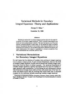
(a) Reference

(e) Initial Difference

(b) Template

(c) Initial Difference

(f) Intensity-Biased

(d) Difference

(g) Intensity-Unbiased

Figure 1: Upper Row: Illustration of the biased behaviour of the unmodified SSD approach on a synthetic “coffee bean”. (a) and (b) are the input images for the registration. The initial difference is presented in (c) and (d) shows the result of the algorithm. Due to the intensity values, the convergence is faster in the left-hand side of the “bean”. This way, the regularizer is saturated by displacements which result mostly from high gradient regions of the image. This behaviour we refer to as intensity-biased. Lower Row: Comparison of the registration results on medical data. The images present differences between reference image R and the template T . (a) Initial difference image. Notice the large intensity differences at the border of the patient; (b) Difference after the unmodified SSD-based approach. While the large displacement at the border of the patient is registered well, the displacement inside the patient is not corrected with the SSD-based approach due to low intensity differences and gradients; (c) Difference after registration with our intensity-unbiased modification. The displacements inside the patient are also corrected. An interpretation of the Euler-Lagrange equation is helpful as a motivation for the method we propose in this paper. The operator A can be seen as describing a reaction of a body, in our case the image, to a set of forces f . It relates the forces f to the deformation ϕ. The acting force f is computed by the derivation of the Euler-Lagrange equations from the dissimilarity term D. As shown in Figure 1, the force resulting from the SSD dissimilarity term is highly biased depending on the intensity values of the two input images. At a certain point, the force depends on the gradient of one of the images and the difference of the two images at this point. Together this leads to large forces at high gradients and large image differences. Hence, the unmodified use of the SSD implies the assumption that objects evolve differently depending on their intensity and background. This would mean that for example bright objects in front of a dark background move or deform more than darker objects. We

refer to this behaviour as intensity-biased. A basic illustration of the problem is presented in Figure 1 on synthetic images and an example from a medical domain. For some applications like morphing where the only goal is to make the images look similar, this is not a real drawback. Small intensity differences are not very noticeable, hence they do not have to be corrected as much as the larger ones. However if physical quantities like real motion are estimated from the results, the intensity-bias problem becomes crucial. In these applications, not the appearance is important but the correctness of the underlying displacement field. In many settings there is no reason why an intensity-biased assumption should be made. Besides not being justified for many applications, this assumption has several drawbacks. As shown in Figure 1 it can lead to slow convergence in certain areas with low gradients and/or low intensity differences between the reference and the template image. A consequence is that the regularizer is saturated by displacements resulting from the image regions with faster convergence. Thus the minimum solution of Equation (1) tends to be biased towards the regions of the image with high intensity differences. In practice these drawbacks are present in many medical imaging modalities such as the computed tomography (CT) shown in Figure 1, where high gradients and intensity differences are present mostly on the boundary of the patient. The actually interesting regions however, are inside the patient and most often have a rather similar intensity. To the best of our knowledge, this drawback of the SSD for respective applications has not yet been addressed in the literature. We state that for the registration task the result should not be dependent on the particular intensity values of the input images at one point, that is the gradient and the intensity difference. This way, although the method stays intensity-based, it becomes intensityunbiased. Instead of computing the forces directly from the Euler-Lagrange equations corresponding to the SSD, we suggest to perform the computation of the force directions and the computation of the force magnitude independently. Using this approach, we modify the standard SSD method in order to establish a simple method which is intensityunbiased. The developped algorithm can be seen in the framework of ”‘demons”’ registration by Thirion [8]. With this modification, the direction of the forces is the same as with the standard unmodified SSD-based approach. The magnitude of the force vectors however is computed independently. The magnitude is not based on the intensity difference and the gradient at one point but it is computed according to the structure of the neighbourhood of the point. This way, the actual displacement of the image point, which can be estimated from the local neighbourhood, influences the magnitude of the force at that point rather than only the information at that point. Some work that might be regarded as similar is the research on robust estimation of optical flow. To this end, several different error measures for the difference of the images have been proposed, see for example [2]. Among these measures is also the L1 norm, which results in the sum of absolute differences (SAD) dissimilarity measure when applied to the difference of the images. While the SAD is less intensity-biased than the SSD because the magnitude of the force is independent on the difference of the images, there is still a bias present based on the magnitude of the gradient. Furthermore, the motivation for the SAD in the context of robust estimation is not to remove the bias but to weigh the outliers less heavily. One other difference is that the work on robustness

is performed on the level of the energy functional while the approach presented here modifies the forces on the level of the Euler-Lagrange equations.

2

Method

This section presents a simple and efficient method which can be used for the separate computation of the direction and the magnitude of forces for variational algorithms. First however, we briefly introduce the used methods and notation.

2.1

Definitions and Problem Setting

The standard methods for deformable registration used in the following are described in detail in the literature, for example in [6, 1, 7, 4]. We define an image I to be a mapping I : Ω → B from a respective functional space H from the d-dimensional image domain Ω = [0, 1]d ⊂ Rd to a bounded interval of real numbers B = [0, 1] ⊂ R. For our applications the dimension is restricted to d = 2, 3. In the following, we consider the registration task of deforming the template image T such that it becomes similar to the reference image R. The deformation is described by the deformation function ϕ, which is a combination of the identity mapping Id and a displacement field u, such that ϕ = Id + u. Here, ϕ, Id and u are all functions from a space F, with F = { f | f : Ω → Ω}. For the computation of the deformation function we define an energy functional I : H × H × F → R to be minimized as I [R, T, ϕ] = D[R, T, ϕ] + αS [ϕ] .

(1)

Here I consists of a dissimilarity term D and a regularizer, also known as smoothing operator, S whose influence is governed by a scalar parameter α ∈ R, α ≥ 0. As a dissimilarity measure we use the SSD measure 1 (R(x) − T (ϕ(x)))2 dx . (2) 2 Ω For the regularizer component S many different terms can be used. The actual regularizer component is not essential for the following since the problem is not restricted to the choice of one special regularization term. The most simple term is the isotropic homogeneous diffusion term and it is used in this paper. It is defined as DSSD [R, T, ϕ] =

S [ϕ] =

Z

Z

d

∑ |∇x ϕi (x)|2 dx = Ω i=1

Z

d

∑ h∇x ϕi (x), ∇x ϕi (x)i dx Ω

,

(3)

i=1

where ∇x is the spatial gradient operator ∂ /∂ x and h·, ·i denotes the scalar product. With this choice of dissimilarity and regularizer component, this model represents the well-known Horn and Schunck approach [5]. In order to minimize the functional I we first have to derive the Euler-Lagrange equation. The deformation function which solves this equation is set to be the solution of the registration problem. Because of the linearity of the functional, the Euler-Lagrange equations can be derived independently for the dissimilarity and the regularization term. The Euler-Lagrange equation derived from the dissimilarity component D is

fSSD (ϕ)(x) = − [R(x) − T (ϕ(x))] ∇x T (ϕ(x)) ,

(4)

and will also be referred to as force. This paper deals with the modification of this term.1 The Euler-Lagrange equation resulting from the regularizer S is A(ϕ)(x) = ∆ϕ(x) ,

(5)

with ∆ being the Laplacian operator.2 The resulting Euler-Lagrange equation for the functional I can be expressed using the differential operators A and f as −αA(ϕ)(x) = f (ϕ)(x) .

(6)

Here f stands for a force term corresponding to a chosen dissimilarity measure, such as fSSD or fSAD defined in the following. Using a discretization technique such as the standard finite difference scheme we obtain the discretized form of the upper equation. This non-linear partial differential equation is usually solved by a gradient descent method which is also the approach we take here [1]. Furthermore we can employ a Gaussian resolution pyramid in order to allow for larger displacements [1]. Since we compare the method presented in this paper also to the SAD-based approach, we present the definition of the SAD DSAD [R, T, ϕ] =

Z

|R(x) − T (ϕ(x))| dx ,

(7)

Ω

as well as the corresponding Euler-Lagrange equation fSAD (ϕ)(x) = −

R(x) − T (ϕ(x)) ∇x T (ϕ(x)) . |R(x) − T (ϕ(x))|

(8)

This SAD-based force can be used as an alternative to the SSD-based term.

2.2

Modification of the Force Term

If we take a closer look at the Equation (4) we can see that two factors influence the magnitude of the forces. The main part of the SSD-based force term used in (4) is [R(x) − T (ϕ(x))] ∇x T (ϕ(x)). We see that the force at point x is proportional to the difference between the reference R(x) and the deformed template T (ϕ(x)) at this point. Furthermore, it is proportional to the gradient magnitude of the deformed template image k∇x T (ϕ(x))k at the same point which also depends on the intensities at the point. To sum up, the above properties of the SSD-based measure cause larger forces for large image intensity differences and gradients than for others. Since the forces cause the deformation, this implies the assumption that points with certain intensities are more likely to move than others. The resulting behaviour is illustrated in Figure 1. The same problem occurs for the SAD-based approach. In Equation (8), we can see that although the difference of the intensities is normalized, such that only the sign of the 1 The force term is dependent not only on the point x but also on the images R and T and the deformation function ϕ. However, for the sake of simplicity we will drop these arguments in the following. 2 For scalar-valued functions g : Rd → R, the Laplace operator is ∆g = d ∂ ∑i=1 xi ,xi g. For the vector-valued case, G : Rd → Rm , the Laplace operator is defined component-wise as ∆G = (∆G1 , . . . , ∆Gm )T .

difference influences the force, the bias is still present through the unscaled magnitude of the gradient. Therefore we propose a modification of the standard SSD-based force term in order to be able to perform intensity-unbiased registration. To this end we separate the computation of the direction and the magnitude of the force vectors. In our approach we keep the direction of the vectors computed with the SSD-based method, which is the direction of ∇x T (ϕ). We make this choice since forces at edges of the body, orthogonal to the edges are meaningful and since the force directions do not cause the intensity-biased behaviour. The direction of the forces is then the normalized force fn (x) =

R(x) − T (ϕ(x)) ∇x T (ϕ(x)) fSSD (x) =− · . k fSSD (x)k |R(x) − T (ϕ(x))| k∇x T (ϕ(x))k

(9)

Regarding the magnitude of the force vectors, several alternatives are possible. We can model these alternatives by introducing a function m : Ω → R which assigns a magnitude to a force at every point of the domain.3 The same general concept for computing the forces with separate terms for direction and magnitiude is used in [8]. This way we get the following modified formula for the computation of the forces f (x) = m(x) fn (x) .

(10)

The most simple alternative for m is to not further modify the force term from Equation (9), that is m(x) = 1, ∀x ∈ Ω. For images without noise this approach works satisfyingly, compare Table 1. In presence of noise however, the forces caused by noise might cause a wrong behaviour, since they have the same magnitude as all other force vectors. One possible approach to this problem might be to assume that the forces caused by random noise will have different directions and thus cancel each other out. This is actually also supported by the regularizer component S used in the method. For some tests, performed with Gaussian and uniform noise of different magnitudes on synthetic images this approach also produced good results. The question is however, how this approach behaves for general images from real applications. In order to develop a more robust approach without having to rely on the quality of noise, a modified method for magnitude computation is needed. The basic idea behind the modification we introduce for the magnitude computation is to make the magnitude dependent not on the values at a single point but on the structure of the neighbourhood of the point. The intuition behind the method is that if large displacements occur, there is a difference between the two input images not only at one point but also in the surrounding area. In order to make this decision intensity-unbiased we are not interested in how large the difference of the intensities is but only if it is present. We implement the above intuition by performing the following steps. First, we compute the difference between the reference and the template image D(x) = R(x) − T (ϕ(x)). In order to make the method more robust in presence of noise, we filter the difference D(x) by a median filter and take the absolute value of the result. In our experiments, this was enough to remove the effects caused by noise. This yields a signal, which is very close to 3 Again, m is dependent on more parameters than only the domain point (R,T ,ϕ) which we drop for simpler notation.

(a) Reference

(b) Template

(c) Initial Difference

(d) Displacement Field

Figure 2: Input for the study on synthetic data. We display the input reference and template images, the initial difference and the displacement field used to generate the template from the reference. The results of the experiments are presented in Table 1 and Figure 3.1. zero in the regions which have no real difference and larger in other regions, depending on the intensities. Now we perform a thresholding step in order to remove the still present bias and set all values below the threshold to 0 and the values above or equal the threshold to 1. This way, the magnitude is no longer dependent on the magnitude of the intensity differences of the two images but only on their existence.

3

Results and Evaluation

We test the proposed method on synthetic and medical 2D data. While the medical data confirm the practicability of the proposed method for real applications, the synthetic test allow us a quantitative evaluation. We use a gradient descent approach in order to overcome the non-linearity of the deformable registration problem [1] and a homogeneous isotropic regularization term for all experiments. For the solution of the arising algebraic linear systems we employ a multigrid solver [3]. The algorithm is implemented in Matlab with no performance tuning. The runtime for one iteration step (computing forces, solving the linear system and applying the deformation) of the gradient descent method is approximately 0.75 seconds for a 2562 image. The runtime overhead needed for the proposed method is approximately 10-15%. For the comparison of the different methods we try to set the parameters as similar as possible in order to achieve a fair evaluation. For all methods we use the same regularization parameter α = 1.0, the same number of iterations, which are sufficient for convergence of all methods, and we scale the forces, such that the resulting mean force magnitude is approximately the same for all methods.

3.1

Evaluation on Medical Data

The medical data used for this experiment are 2D slices from an abdominal CT scan. Because in this case we deal with real data we have no ground truth displacement. So we can only perform a qualitative comparison of the different methods. We compare the SSD-based method and our approach by visual inspection of the difference images between the reference R and the deformed template image T after the registration process. We can see a clear improvement in small gradient and low intensity

(a) SSD-based

(b) SAD-based

(c) modified

(d) SSD-based

(e) SAD-based

(f) modified

Figure 3: Comparison of the results on synthetic data with 10% uniform noise. The input data is shown in Figure 2. The upper row presents the difference images after the respective algorithms. Please notice that the maximal errors are lower for the modified method (range:0-0.25) than for the SSD and SAD-based approaches (range: 0-0.45). The lower row illustrates the improvement in the displacement field by displaying the norm of the error fields, compare also Table 1. Here the black values mean that the error of the computed displacement is low. Clearly, the modified intensity-unbiased approach performs better than the SSD and the SAD-based method in the inner area with low intensity differences and low gradients. Of course, the error stays large for all methods in regions with no structure. difference areas when using our method. The results are displayed in Figure 1. The registration in this experiment is performed using a Gaussian resolution pyramid.

3.2

Evaluation on Synthetic Data

Comparison of difference images has a drawback that only the apparent similarity is compared - small intensity differences are not visible. For our purposes however, it is more important to examine the computed displacement fields. In order to be able to perform this quantitative evaluation of the proposed method, we use synthetic data sets. We employ a ground truth displacement field in order to compute the template from the reference image and we also use this synthetic setting to test the methods in presence of noise. We compare the performance of the standard SSD-based method, the SAD-based method, the simple modification where all force magnitudes are normalized to unity and finally our approach.

Results on Image mean no noise std. dev. mean 10% uniform std. dev. mean 20% uniform std. dev.

SSD 1.3671 1.5760 1.3802 1.5839 1.3890 1.5918

SAD 1.1311 1.2636 1.1605 1.2666 1.2010 1.3232

Unit Force 0.9525 1.1066 1.5652 1.2098 1.5693 1.2286

Our Method 0.9793 1.1371 1.0047 1.1634 1.1471 1.2216

Results on ROI mean no noise std. dev. mean 10% uniform std. dev. mean 20% uniform std. dev.

SSD 3.2495 1.4085 3.2639 1.1500 3.2798 1.4202

SAD 2.5384 1.1965 2.5792 1.2015 2.7180 1.2494

Unit Force 2.0943 1.1692 2.4610 1.3454 2.6505 1.3602

Our Method 2.2077 1.1288 2.2448 1.1833 2.4385 1.2561

Table 1: Quantitative results of the phantom study. The upper table shows the results for the complete image, the lower for the region of interest inside the phantom where the low intensity differences and gradients are dominating. We compute the norm of difference between the ground truth uGT and the estimated displacement field u and give the mean value and the standard deviation of kuGT − uk. The mean of the uGT is 3.5459 with a standard deviation of 1.5477. The methods tested are the SSD and SAD-based approach, the simple modification with forces normalized to unity and our intensity-unbiased modification. Tests were performed with no noise and with 10% and 20% uniform noise. The modified method presents a clear improvement over both the SSD and the SAD-based approach. All values are in pixel units. The used images are generated with the Matlab inbuilt phantom function and the displacement field is a combination of Gaussians in each dimension, see Figure 2. For experiments with noise with use a uniform noise in range of 10% and 20% of the maximal image intensities, that is [0, 0.1] and [0, 0.2]. For the experiments we do not use a Gaussian pyramid since we want to isolate the behaviour of the methods and the pyramid implicitly influences the results in presence of noise by smoothing on the low-resolution levels. We compare the methods by examining the norm of difference field e = kuGT − uk between the ground truth uGT and the displacement field u estimated by the respective method. The error norm is inspected by computing the mean value and the standard deviation of e. The parameters for the proposed approach were determined experimentally. However, they did not have to be changed during the tests. The size of the neighbourhood for the median filter is 5 × 5 and the threshold is ε = 0.025. The results of the experiments are summarized in Table 1 and Figure 3.1. We can see a clear improvement of the error of the displacement field with our method in regions with low intensity differences and small gradients. This leads to an overall better performance of our approach. The simple force-normalizing approach performs well for the case with no noise, however it is very sensitive to noise in the homogeneous areas.

4

Summary and Further Work

We address the problem of the intensity-bias of the SSD measure for variational motion estimation methods. The proposed solution separates the computation of the direction and the magnitude of the forces, which are usually yielded from the Euler-Lagrange equations corresponding to the SSD. While we keep the direction of the forces, we modify the magnitude in such way that it is not biased to large intensity differences or high gradients. The robustness is improved by setting the magnitude to zero in regions where the forces are resulting only from the presence of noise and not from real deformations. The proposed method is tested on 2D synthetic images and real medical data and shows a better performance than the standard SSD and SAD-based techniques. Our further work on this topic will include an integration of the methods presented here into an existing framework for deformable registration of 3D medical images. Furthermore, we plan to investigate the behaviour of other dissimilarity measures like the Cross-Correlation, Correlation Ratio and Mutual Information with respect to the problem of the intensity-bias.

References ´ [1] Luis Alvarez, Joachim Weickert, and Javier S´anchez. Reliable estimation of dense optical flow fields with large displacements. International Journal of Computer Vision, 39(1):41–56, 2000. [2] Michael J. Black and P. Anandan. A framework for the robust estimation of optical flow. In Fourth International Conference on Computer Vision, pages 231–236, 1993. [3] Andr´es Bruhn, Joachim Weickert, Christian Feddern, Timo Kohlberger, and Christoph Schn¨orr. Variational optical flow computation in real time. IEEE Transactions on Image Processing, 14(5):608–615, 2005. [4] Gerardo Hermosillo. Variational Methods for Multimodal Image Matching. PhD thesis, Universit´e de Nice - Sophia Antipolis, 2002. [5] Berthold K.P. Horn and Brian G. Schunck. Determining optical flow. Technical report, Cambridge, MA, USA, 1980. [6] Jan Modersitzki. Numerical methods for image registration. Oxford University Press, 2004. [7] Christoph Schn¨orr and Joachim Weickert. Variational image motion computation: Theoretical framework, problems and perspectives. In Gerald Sommer, Norbert Kr¨uger, and Christian Perwass, editors, DAGM-Symposium, Informatik Aktuell, pages 476–488. Springer, 2000. [8] J.P. Thirion. Image matching as a diffusion process: an analogy with maxwells demons. Medical Image Analysis, 2(3):243–260, 1998.