Interaction Control of Robot Manipulators Using Force and Vision

Interaction Control of Robot Manipulators Using Force and Vision Vincenzo Lippiello, Bruno Siciliano, Luigi Villani PRISMA Lab Dipartimento di Informatica e Sistemistica Universit` a degli Studi di Napoli Federico II Via Claudio 21, 80125 Napoli, Italy {lippiell,siciliano,lvillani}@unina.it Abstract. An approach to force and visual control of robot manipulators in contact with a partially known environment is proposed in this paper. The environment is modelled as a rigid object of known geometry but of unknown and time-varying position and orientation. An algorithm for online estimation of the object pose is adopted, based on visual data provided by a camera as well as on forces measured during the interaction. This information is used by a force/position control scheme, in charge of managing the interaction. Simulation and experimental results are presented for the case of an industrial robot manipulator.

1 Introduction The autonomy of a robotic system is strictly connected to the availability of sensing information on the external environment; among the various sensing capabilities, vision and force play a fundamental role. In fact, visual perception allows achieving global information on the surrounding environment to be used for task planning and obstacle avoidance. On the other hand, the perception of the force applied to the end effector of a robot manipulator allows adjusting the end-effector motion so that the local constraints imposed by the environment during the interaction are satisfied. Several approaches to control of robot manipulators combining force and vision feedback have been developed so far, e.g., hybrid visual/force control (Hosoda et al., 1998), shared and traded control (Nelson et al., 1995; Baeten and De Schutter, 2004) or visual impedance control (Morel et al., 1998; Olsson et al., 2004). These algorithms improve classical interaction control schemes (Siciliano and Villani, 1999), e.g., impedance control, hybrid force/position control, parallel force/position control, where only force and joint position measurements are used. A comparison of different control algorithms combining force and vision can be found in (Deng et. al, 2005).

2

Vincenzo Lippiello, Bruno Siciliano, Luigi Villani

In general, interaction control approaches require knowledge of the geometry of the environment in the form of constraints imposed to the endeffector motion. Some of these approaches, like hybrid force/position control (Yoshikawa et al., 1988), make explicit use of the constraint equations for the design of the control law; other approaches, like impedance control (Hogan, 1985) and parallel force/position control (Chiaverini and Sciavicco, 1993), exploit the available knowledge of the geometry of the environment for the selection of the control gains and the choice of the reference force and position trajectories. In the framework presented in this paper, the geometry of the environment is assumed to be known, but its position and orientation with respect to the robot end-effector are unknown. The relative pose is estimated online from all the available sensor data, i.e., visual, force and joint position measurements, using the Extended Kalman Filter (EKF). The estimated pose is then exploited for computing online the constraint equations used by standard interaction control laws. Differently from the approaches reported in (Deng et al., 2005), the resulting scheme has an inner/outer control structure where the inner control loop is a standard interaction control law based of joint positions and force feedback, while the outer loop exploits all the available measurements, i.e., joint positions, force and vision, to estimate the relative pose of the environment with respect to the robot. The pose estimation algorithm is an extension of the visual tracking scheme proposed in (Lippiello and Villani, 2003) to the case that also force and joint position measurements are used. Remarkably, the same algorithm can be adopted both in free space and during the interaction, simply modifying the measurements set of the EKF. The approach presented here was developed in previous conference papers (Lippiello et al., 2007a; Lippiello et al., 2007b), for the case of impedance control and hybrid force/position control respectively. Two case studies on an industrial robot are considered. Simulation results are reported for the case of an hybrid force/position control scheme, while experimental tests are presented for the case of impedance control.

2 Modelling Consider a robot in contact with an object, a wrist force sensor and a camera mounted on the end effector (eye-in-hand) or fixed in the workspace (eye-tohand). In this Section, some modelling assumptions concerning the object, the robot and the camera are presented. 2.1 Object The position and orientation of a frame Oo –xo yo zo attached to a rigid object with respect to a base coordinate frame O–xyz can be expressed in terms of the coordinate vector of the origin oo and of the rotation matrix Ro (ϕo ),

Interaction Control of Robot Manipulators Using Force and Vision

3

where ϕo is a (p × 1) vector corresponding to a suitable parametrization of the orientation. In the case that a minimal representation of the orientation is adopted, e.g., Euler angles, it is p = 3, while it is p = 4 if unit quaternions T are used. Hence, the (m × 1) vector xo = [ oT ϕT o o ] defines a representation of the object pose with respect to the base frame in terms of m = 3 + p parameters. ˜ = [ pT 1 ]T of a point P of the The homogeneous coordinate vector p ˜ = H o (xo )op ˜, object with respect to the base frame can be computed as p o˜ where p is the homogeneous coordinate vector of P with respect to the object frame and H o is the homogeneous transformation matrix representing the pose of the object frame referred to the base frame. It is assumed that the geometry of the object is known and that the interaction involves a portion of the external surface which satisfies a twice differentiable scalar equation ϕ(op) = 0. Hence, the unit vector normal to the surface at the point op and pointing outwards can be computed as: o

n(op) =

(∂ϕ(op)/∂ op)T , k(∂ϕ(op)/∂ opk

(1)

where o n is expressed in the object frame. Notice that the object pose xo is assumed to be unknown and may change during the task execution. As an example, a compliant contact can be modelled assuming that xo changes during the interaction according to an elastic law. A further assumption is that the contact between the robot and the object is of point type and frictionless. Therefore, when in contact, the tip point Pq of the robot instantaneously coincides with a point P of the object, so that the tip position opq satisfies the surface equation ϕ(opq ) = 0. Moreover, the (3 × 1) contact force o h is aligned to the normal unit vector o n. 2.2 Robot The case of a n-joints robot manipulator is considered, with n ≥ 3. The tip position pq can be computed via the direct kinematics equation pq = k(q), where q is the (n × 1) vector of the joint variables. Also, the velocity of the robot’s tip v Pq can be expressed as v Pq = J (q)q˙ where J = ∂k(q)/∂q is the robot Jacobian matrix. The vector v Pq can be decomposed as o

v Pq = op˙ q + Λ(o pq )o ν o ,

(2)

with Λ(·) = [ I 3 −S(·) ], where I 3 is the (3 × 3) identity matrix and S(·) denotes the (3 × 3) skew-symmetric matrix operator. In Eq. (2), op˙ q is the relative velocity of the tip point Pq with respect to the object frame while T o ν o = [ o v TOo o ω To ] is the velocity screw characterizing the motion of the object frame with respect to the base frame in terms of the translational velocity of the origin v Oo and of the angular velocity ωo . When the robot is

4

Vincenzo Lippiello, Bruno Siciliano, Luigi Villani

in contact with the object, the normal component of the relative velocity op˙ q is null, i.e., o nT (opq )op˙ q = 0. 2.3 Camera A frame Oc –xc yc zc attached to the camera is considered. By using the classical T pin-hole model, a point P of the object with coordinates c p = [ x y z ] with respect to the camera frame is projected onto the point of the image plane with coordinates [ X Y ]T = λc [ x/z y/z ]T where λc is the lens focal length. The homogeneous coordinate vector of P with respect to the camera frame ˜ = cH o (xo , xc )o p ˜ . Notice that xc is constant for eyecan be expressed as c p to-hand cameras; moreover, the matrix cH o does not depend on xc and xo separately but on the relative pose of the object frame with respect to the camera frame. The velocity of the camera frame with respect to the base frame can be characterized in terms of the translational velocity of the origin v Oc and of angular velocity ω c . These vectors, expressed in camera frame, define the T velocity screw c ν c = [ c v TOc c ω Tc ] . It can be shown that the velocity screw c c T c T T ν o = [ v Oo ω o ] corresponding to the absolute motion of the object frame can be expressed as c

ν o = c ν o,c + Γ (c oo )c ν c

(3)

T where c ν o,c = [ c o˙ To c ω To,c ] is the velocity screw corresponding to the relative motion of the object frame with respect to camera frame, and the matrix Γ (·) is   I 3 −S(·) Γ (·) = , O3 I3

being O 3 the (3 × 3) null matrix. The velocity screw r ν s of a frame s with respect to a frame r can be expressed in terms of the time derivative of the vector xs representing the pose of frame s through the equation r

ν s = r L(xs )x˙ s

(4)

where r L(·) is a Jacobian matrix depending on the particular choice of coordinates for the orientation.

3 Object pose estimation When the robot moves in free space, the unknown object pose can be estimated online by using vision; when the robot is in contact with the target object, also the force measurements and the joint position measurements can

Interaction Control of Robot Manipulators Using Force and Vision

5

be used. In this Section, the equations mapping the measurements to the unknown position and orientation of the object are derived. Then, the estimation algorithm based on the EKF is presented. 3.1 Vision Vision is used to measure the image features, characterized by a set of scalar parameters fj grouped in a vector f = [ f1 · · · fk ]T . The mapping from the position and orientation of the object to the corresponding image feature vector can be computed using the projective geometry of the camera and can be written in the form f = g f (cH o (xo , xc )), (5) where only the dependence from the relative pose of the object frame with respect to camera frame has been explicitly evidenced. For the estimation of the object pose using EKF, it is required the computation of the Jacobian matrix J f = ∂g f /∂xo . To this purpose, the time derivative of (5) can be computed in the form ∂g f ∂g f f˙ = x˙ o + x˙ c , (6) ∂xo ∂xc where the second term in the right hand side is null for eye-to-hand cameras. On the other hand, the time derivative of (5) can be expressed also in the form f˙ = J o,c c ν o,c where the matrix J o,c is the Jacobian mapping the relative velocity screw of the object frame with respect to the camera frame into the variation of the image feature parameters. The expression of J o,c depends on the choice of the image features; examples of computation can be found in (Espiau et al., 1992). Taking into account the velocity composition (3), vector f˙ can be rewritten in the form f˙ = J o,c c ν o − J c c ν c

(7)

where J c = J o,c Γ (c oo ) is the Jacobian corresponding to the contribution of the absolute velocity screw of the camera frame, known in the literature as interaction matrix (Espiau et al., 1992). Considering Eq. (4), the comparison of (7) with (6) yields J f = J o,c c L(xo ). (8) 3.2 Force In the case of frictionless point contact, the measure of the force h at the robot tip during the interaction can be used to compute the unit vector normal to the object surface at the contact point opq , i.e., nh = h/khk.

(9)

6

Vincenzo Lippiello, Bruno Siciliano, Luigi Villani

On the other hand, vector nh can be expressed as a function of the object pose xo and of the robot position pq in the form nh = Ro on(opq ) = g h (xo , pq ),

(10)

being opq = RTo (pq − oo ). For the estimation of the object pose, it is required the computation of the Jacobian matrix J h = ∂g h /∂xo . To this purpose, the time derivative of (10) can be expressed as n˙ h = but also as o

∂g h ∂g h x˙ o + p˙ , ∂xo ∂pq q

(11)

˙ o o n(op ) + Ro oN (op )op˙ , n˙ h = R q q q o

o

o

(12) o˙

where N ( pq ) = ∂ n/∂ pq depends on the surface curvature and pq can be computed as
o ˙ q − o˙ o + S(pq − oo ω o ). p˙ q = RT o p

Hence, replacing the above expression in (12) and taking into account the ˙ o o n(op ) = −S(nh )ω o , the following equality holds: equality R q
n˙ h = N p˙ q − N o˙ o − S(nh ) − N S(pq − oo ) ωo

(13)

where N = Ro oN (opq )RTo . Considering Eq. (4), the comparison of (11) with (13) yields J h = − [ N S(nh )−NS(pq −oo ) ] L(xo ). (14) 3.3 Joint positions The measurement of the joint position vector q can be used to evaluate the position of the point P of the object when in contact with the robot’s tip point Pq , using the direct kinematics equation. In particular, it is significant computing the scalar δhq = nTh pq = ghq (xo , pq ),

(15)

using also the force measurements via Eq. (9). This quantity represents the component of the position vector of the robot’s tip point along the constrained direction nh . The corresponding infinitesimal displacement is the same for the robot and for the object (assuming that contact is preserved). This is not true for the other components of the tip position, which do not provide any useful information on the object motion because the robot’s tip may slide on the object surface; therefore, these components are not useful to estimate the pose of the object. The EKF requires the computation of the Jacobian matrix J hq = ∂ghq /∂xo . The time derivative of δhq can be expressed as

Interaction Control of Robot Manipulators Using Force and Vision

∂ghq ∂ghq δ˙hq = x˙ o + p˙ , ∂xo ∂pq q

7

(16)

but also as δ˙hq = n˙ Th pq + nTh Ro (o p˙ q + Λ(o pq )o ν o ) where the expression of the absolute velocity of the point Pq in (2) has been used. Using the identity o T o n ( pq )op˙ q = 0, this equation can be rewritten as δ˙hq = pTq n˙ h + nTh Λ(pq − oo )ν o .

(17)

Hence, comparing (16) with (17) and taking into account (12), (14) and (4), the following expression can be found J hq = pTq J h + nTh Λ(pq − oo )L(xo ).

(18)

3.4 Extended Kalman Filter The pose vector xo of the object with respect to the base frame can be estimated using an Extended Kalman Filter. To this purpose, a discrete-time state space dynamic model has to be considered, describing the object motion. The state vector of the dynamic model T is chosen as w = [ xT x˙ T o o ] . For simplicity, the object velocity is assumed to be constant over one sample period Ts . This approximation is reasonable in the hypothesis that Ts is sufficiently small. Hence, the discrete-time dynamic model can be written as wk = Awk−1 +γ k , where γ is the dynamic modelling error described by zero mean Gaussian noise with covariance Q and A is the (2m × 2m) block matrix   I m Ts I m A= . Om Im The output of the EKF, in the case that all the available data can be used, T is the vector ζ k = [ ζ Tf,k ζ Th,k ζhq,k T ] of the measurements at time kTs , where ζ f,k = f k + µf,k , ζ h,k = hk + µh,k , and ζhq,k = δk + µhq,k , being µ the measurement noise, which is assumed to be zero mean Gaussian noise with covariance Π. Taking into account the Eqs. (5), (10), and (15), the output equation of T the EKF can be written as ζ k = g(w k ) + µk , with [ µTf,k µTh,k µThq,k ] and T T T T g(w k ) = [ g f (w k ) g h (wk ) ghq (wk ) ] , where only the explicit dependence on the state vector wk has been evidenced. The EKF requires the computation of the Jacobian matrix of the output equation   ∂g(w) ∂g(w) Ck = = , O ∂w w=w ∂xo ˆ k,k−1 ˆ k,k−1 w =w

where O is a null matrix of proper dimensions corresponding to the partial derivative of g with respect to the velocity variables. The Jacobian matrix

8

Vincenzo Lippiello, Bruno Siciliano, Luigi Villani

∂g(w)/∂xo , in view of (8), (14), and (18) has the expression ∂g(w)/∂xo = T [ J Tf J Th J Thq ] . The equations of the recursive form of the EKF are standard and are omitted here and can be found, e.g., in (Lippiello and Villani, 2003). Notice that the adoption of the unit quaternion to represent the object orientation allows avoiding the problems of representation singularities typical of three-parameters representations. However, in the implementation of the Kalman filter, the unit norm constraint must be enforced to the estimated quaternion using, e.g., simple vector normalization (Choukroun et al., 2006).

4 Interaction control The proposed algorithm can be used to estimate online the pose of an object in the workspace; this allows computing the surface equation with respect to the base frame in the form ϕ(RT o (pq − oo )) = ϕ(q, t) = 0, where the last equality holds in view of the direct kinematic equation of the robot. In the following, it is assumed that the object does not move; the general case of moving object is more complex but can be analyzed in a similar way. Hence, the constraint equation is ϕ(q) = 0; moreover J ϕ (q)q˙ = 0, where J ϕ = ∂ϕ/∂q is a (1 × n) vector. The dynamic model of the manipulator in contact with the environment is ˙ = τ − JT B(q)¨ q + n(q, q) ϕ (q)λ, ˙ where B is the (n × n) symmetric and positive definite inertia matrix, n(q, q) is the (n × 1) vector taking into account Coriolis, centrifugal, friction and gravity torques, τ is the (n × 1) vector of the joint torques, and λ is the lagrangian multiplier associated to the constraint. The online computation of the constraint equations can be suitably exploited for interaction control. In the following, the case of the hybrid force/position control and of the impedance control are considered. 4.1 Hybrid force/position control Following the formulation presented in (Villani and De Shutter, 2008) the configuration of the robot subject to the constraint ϕ(q) = 0 can be described in terms of a suitable vector r of (n − 1) independent variables. From the implicit function theorem, this vector can be defined as r = ψ(q), where ψ(q) is any ((n − 1) × 1) twice differentiable vector function such that the (n−1) components of ψ(q) and function ϕ(q) are linearly independent at least locally in a neighborhood of the operating point. This implies the existence of a (n × 1) vector function ρ(r) such that q = ρ(r), at least locally. Moreover, the Jacobian J ρ = ∂ρ/∂r of the differential mapping q˙ = J ρ (r)r˙ is a full-rank matrix. The matrices

Interaction Control of Robot Manipulators Using Force and Vision Desired Task

rd

Dynamic Trajectory Planner

ld

Hybrid Force/Position Control

9

Target Object

Robot

Joint feedback (1khz)

Force feedback (1khz)

Pose feedback

Pose Estimation

(50hz)

Images

Visual System

Fig. 1. Hybrid force/position control.

S f = J −T (q)J T ϕ (q),

S v = J(q)J ρ (r),

˙ play the role of selection by virtue of the equalities h = S f λ and v Pq = S v r, matrices. An hybrid force/position control task can be assigned by specifying the desired force λd (t) and the n − 1 components of the vector r d (t). An inverse dynamics control law can be adopted, by choosing the control torque τ as ˙ q˙ + J T τ = B(q)α + n(q, q) ϕ (q)S f hλ , ˙ with α = J −1 (q)(S v αv + S˙ v r˙ − J˙ q), ¨d + K Dr (r˙ d − r) ˙ + K P r (r d − r) αv = r and hλ = λd + kIλ

Z

(19)

t

(λd (τ ) − λ(τ ))dτ,

(20)

0

where K Dr , K P r and kIλ are suitable feedback gains. From the block scheme of Fig. 1 it can be observed that the algorithm has a inner/outer structure, where the inner loop implements hybrid control whereas the outer loop computes the estimation of the object pose as well as the desired force and motion trajectories, on the basis of force, joint and visual measurements. Usually, the outer loop runs at a frequency lower than the inner loop, due to the limitation in the maximum camera frame rate (between 25 Hz and 60 Hz for low-cost cameras used in standard applications). 4.2 Impedance Control The above scheme can be easily modified by replacing the inner hybrid force/position control with a different interaction control scheme. For instance, a position-based impedance control algorithm, based on the concept of compliant frame (Siciliano and Villani, 1999), can be adopted (see Fig. 2).

10

Vincenzo Lippiello, Bruno Siciliano, Luigi Villani Pose Control Desired Task

Dynamic Trajectory Planner

Impedence Control

Target Object

Robot

Joint feedback (1khz)

Force feedback (1khz)

Pose feedback (26hz)

Pose Estimation Visual System

Fig. 2. Position-based visual impedance control.

In detail, on the basis of the current estimate of the constraint equation, the Dynamic Trajectory Planner generates a pose trajectory for a desired end-effector frame specified in terms of the position of the origin pd and orientation matrix Rd . Moreover, a compliant frame r is introduced, specified in terms of pr and Rr . Then, a mechanical impedance between the desired and the compliant frame is considered, so as to contain the values of the interaction force h and moment m. In other words, the desired position and orientation, together with the measured contact force and moment, are input to the impedance equation which, via a suitable integration, generates the position and orientation of the compliant frame to be used as a reference for the motion controller of the robot end effector. As far as the compliant frame is concerned, the position pr can be computed via the translational impedance equation M p ∆¨ pdr + D p ∆p˙ dr + K p ∆pdr = h,

(21)

where ∆pdr = pd − pr , and M p , Dp and K p are positive definite matrices representing the mass, damping, and stiffness characterizing the impedance. The orientation of the reference frame Rr is computed via a geometrically consistent impedance equation similar to (21), in terms of an orientation error based on the (3 × 1) vector r ǫdr , defined as the vector part of the unit quaternion that can be extracted from r Rd = RTr Rd . The corresponding mass, damping and inertia matrices are M o , D o and K o respectively. More details about the geometrically consistent impedance based on the unit quaternion can be found in (Siciliano and Villani, 1999). It is interesting noticing that the above scheme is able to manage both contact and free-space motion phases. In fact, during free space motion, the position-based impedance control is equivalent to a pose control and the whole scheme corresponds to a classical position-based visual servoing algorithm (Lippiello et al., 2007c). For this reason, this scheme can be classified as position-based visual impedance control.

Interaction Control of Robot Manipulators Using Force and Vision

11

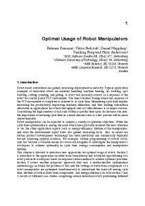
Fig. 3. Experimental setup.

5 Case studies The proposed approach has been tested in a number of simulation and experimental case studies. The setup (Fig. 3) is composed by a 6-DOF industrial robot Comau SMART-3 S with an open control architecture based on RTAILinux operating system. A six-axis force/torque sensor ATI FT30-100 with force range of ±130 N and torque range of ±10 N·m is mounted at the arm’s wrist, providing readings of six components of generalized force at 1 ms. A visual system composed by a PC equipped with a Matrox GENESIS board and a Sony 8500CE B/W camera is available. The camera is fixed and calibrated with respect to the base frame of the robot. 5.1 Hybrid force/position control A simulation study has been developed to test the hybrid force/position control scheme. The MATLAB/Simulink kinematic and dynamic models of the Comau SMART-3 S can be found in (Siciliano and Villani, 1999). A planar object surface is considered, described by the equation o nT o p = 0, assuming that the origin Oo of the object frame is a point of the plane and the axis zo is aligned to the normal o n. During the interaction with the robot, the normal vector n remains constant in the base frame while the plane is assumed to be elastically compliant along n according to a simple elastic law. The contact force of the object on the robot’s tip at pq is given by  knnT (po − pq ) if nT (po − pq ) ≥ 0 h= 0 if nT (po − pq ) < 0 where pq is on the plane when h 6= 0 while po is a constant vector representing the position of a point of the plane when h = 0. The scalar k, representing the stiffness of the surface, has been set to 10000 N/m.

12

Vincenzo Lippiello, Bruno Siciliano, Luigi Villani

x y

m

z sec

sec Fig. 4. Pose estimation error in the first simulation. Top: position error; bottom: orientation error.

y x y

N

Nm

z

z x

sec

sec

Fig. 5. Measured force (left) and moment (right) in the first simulation.

The end-effector tool is a rigid stick of 25 cm length. The robot has a force/torque sensor mounted at the wrist. Neglecting the weight and inertia of the tool, the force at the robot’s tip pq and that measured at the robot wrist by the force sensor are the same, while a moment is measured by the sensor if the stick is not aligned to o n. A camera is mounted on the robot end effector. It is assumed that the intrinsic parameters of the camera are affected by a 3% error, while the extrinsic parameters are supposed to be known with a tolerance of ±1 cm for the position and ±3 deg for the orientation. The object features are 4 points at the corners of a square of 10 cm side. The control parameters in (19) and (20) are chosen as: K P r = diag{250, 250, 250, 15, 15, 15}, K Dr = diag{220, 220, 220, 10, 10, 10} and kIλ = 0.05; a 1 ms sampling time has been selected. These values have been selected by imposing a given closed-loop bandwidth and damping.

Interaction Control of Robot Manipulators Using Force and Vision

13

x z

m y

sec

sec Fig. 6. Pose estimation error in the second simulation. Top: position error; bottom: orientation error.

x y y

N

z

Nm

z x

sec

sec

Fig. 7. Measured force (left) and moment (right) in the second simulation.

The desired task is planned in the object frame and consists in a straightline motion of the end effector along the zo axis keeping a fixed orientation with the stick normal to the xo yo plane. The final position is the estimated rest position of the plane. During this phase, only the end-effector position and orientation are controlled, according to the law (19) applied to all the task directions. When force is detected, the motion controller is replaced by the hybrid force/position control law (19) and (20), with a constant position and orientation and a desired force of −20 N along the zo axis. After 2 sec, a desired circular trajectory on the contact plane with 10 cm radius and 8 sec duration is commanded for the end-effector position, while the desired orientation is unchanged and the desired force is kept constant to −20 N. In the EKF, the non null elements of the matrix Π has been set equal to 625·10−11 for f , 10−5 for nh and 10−6 for δhq . These values have been set on the basis of the calibration errors of the camera. The state noise covariance matrix has been selected so as to give a rough measure of the errors due to

14

Vincenzo Lippiello, Bruno Siciliano, Luigi Villani

the simplification introduced in the model (constant velocity), by considering only velocity disturbance, i.e. Q = diag{0, 0, 0, 0, 0, 0, 0, 5, 5, 0.5, 102, 103 , 103 , 103}·10−11. Notice that the unit quaternion has been used for the orientation in the EKF. Moreover a 20 ms sampling time has been set for the estimation algorithm, corresponding to the typical camera frame rate of 50 Hz. Two different simulations are presented, to show the effectiveness of the use of force and joint position measurements, besides visual measurements. In the first simulation, only the visual measurements are used. The object pose estimation errors are reported in Fig. 4. The position error is computed as the difference between the real position of the origin of the objet frame and the estimated position referred to the object frame; the orientation error is defined as the norm of the vector part of the quaternion extracted from the rotation matrix representing the mutual orientation of the real object frame with respect to the estimated frame. The task starts at time to = 0 s, when an estimate of the object pose is available from visual measurements; notice that the initial value of the pose estimation error in non null, due to camera calibration errors and remains different from zero during all the task. The time history of the force and moments measured by the sensor are reported in Fig. 5. Notice that the normal component of the measured force (the z component), after a transient, reaches a value close to the desired one. However, the y component of the force remains non null and a moment different from zero can be observed during the task execution, due to the error in the estimation of zo . The same task is repeated using also the contact force and the joint position measurements for object pose estimation; the results are reported in Fig. 6 and Fig. 7. Before the contact (i.e. before time tc ≃ 2.2 s), the estimation errors are the same as in the previous simulation. After the contact, the benefit of using additional measurements in the EKF results in a significant reduction of the pose estimation error, especially for the z component of the position (aligned to zo ) and for the orientation. The peak of the measured force during the transient is lower than before and the value of the normal component of the force, during the execution of the circle, remains very close to the desired value of −20 N. Finally, all the other components of the measured force, as well as the measured moment, become null after a short transient, meaning that the stick remains aligned to zo . 5.2 Impedance control Experimental tests have been carried out to check the performance the impedance control scheme. The environment is a planar wooden horizontal surface, with an estimated stiffness (along o n) of about 46000 N/m. The object features are 8 landmark points lying on the plane at the corners of two rectangles of 10 × 20 cm size (as in Fig. 3).

Interaction Control of Robot Manipulators Using Force and Vision

x

15

x y

N

Nm z z

y sec

sec

Fig. 8. Measured force (left) and moment (right) in the 1st experiment.

x y N

x Nm z

z

y sec

sec

Fig. 9. Measured force (left) and moment (right) in the 2nd experiment.

The impedance parameters are chosen as: M p = 40I 3 , Dp = 26.3I 3 and K p = 1020I 3 , M o = 15I 3 , Do = 17.4I 3 and K o = 3I 3 ; a 1 ms sampling time has been selected for the impedance and pose control. Notice that the stiffness of the object is much higher that the positional stiffness of the impedance, so that the environment can be considered rigid. The desired task is planned in the object frame and consists in a straightline motion of the end effector along the zo -axis keeping a fixed orientation with the stick normal to the xo yo -plane. The final position is o pf = [ 0 0 0.05 ]T m, which is chosen to have a normal force of about 50 N at the equilibrium, with the selected value of the impedance positional stiffness. A trapezoidal velocity profile time-law is adopted, with a cruise velocity of 0.01 m/s. The absolute trajectory is computed from the desired relative trajectory using the current object pose estimation. The final position of the end effector is held for 2 s; after, a vertical motion in the opposite direction is commanded. In the EKF, the non null elements of the matrix Π have been set equal to 2.5 pixel2 for f , 5·10−4 for nh and 10−6 m2 for δhq . These values have been set

16

Vincenzo Lippiello, Bruno Siciliano, Luigi Villani

on the basis of the calibration errors of the camera. The state noise covariance matrix has been selected so as to give a rough measure of the errors due to the simplification introduced in the model (constant velocity), by considering only velocity disturbance, i.e. Q = diag{0, 0, 0, 0, 0, 0, 0, 10, 10, 10, 1, 1, 1} · 10−9 . Notice that the unit quaternion has been used for the orientation in the EKF. Moreover a 38 ms sampling time has been used for the estimation algorithm, corresponding to the typical camera frame rate of 26 Hz. Two different experiments are presented, to show the effectiveness of the use of force and joint position measurements, besides visual measurements. In the first experiment only the visual measurements are used. The time history of the measured force and moment in the sensor frame are reported in Fig. 8. Notice that the force is null during the motion in free space and becomes different from zero after the contact. The impedance control keeps the force limited during the transient while, at steady state, the force component along the z axis reaches a value of about −65 N, which is different from the desired value of −50 N. This is caused by the presence of estimation errors on the position of the plane due to calibration errors of the camera. Moreover, the moment measured by the sensor is different from zero due to the misalignment between the estimated and the real normal direction of the plane. The same task is repeated using also the contact force and the joint position measurements for object pose estimation; the results are reported in Fig. 9. It can be observed that the benefit of using additional measurements in the EKF results in a force along the vertical direction which is very close to the desired value, due to the improved estimation of the position of the plane; moreover, the contact moment is also reduced because of the better estimation of the normal direction of the plane.

6 Conclusion A framework for force and visual control of robot manipulators was proposed in this paper. The environment was assumed as a rigid object of known geometry but unknown and possibly time-varying position and orientation. An estimation algorithm was adopted, based on visual, force and joint position data, which allows computing the actual position and orientation of the object so as to update in real time the constraint equations for the robot end effector. The resulting control has a inner/outer structure where the outer loop performs pose estimation and the inner loop is an interaction control scheme. Simulation and experimental results have demonstrated the superior performance of the proposed approach with respect to algorithms based on force measurements or visual measurements separately.

Interaction Control of Robot Manipulators Using Force and Vision

17

7 Acknowledgements The research leading to these results has been supported in part by the PHRIENDS specific targeted research project, funded by the European Community’s Sixth Framework Programme under contract IST-045359, and in part by the DEXMART large-scale integrating project, funded by the European Community’s Seventh Framework Programme under grant agreement ICT-216239. The authors are solely responsible for its content. It does not represent the opinion of the European Community and the Community is not responsible for any use that might be made of the information contained therein.

References Baeten, J. and J. De Schutter. 2004. Integrated Visual Servoing and Force Control. The Task Frame Approach. Heidelerg, D: Springer. Chiaverini, S. and L. Sciavicco. 1993. The parallel approach to force/position control of robotic manipulators. IEEE Trans. on Robotics and Automation. 9: 361–373. Choukroun, D., Y. Itzhack, Y. Bar-Itzhack and Y. Oshman. 2006. Novel Quaternion Kalman Filter. IEEE Transactions on Aerospace and Electronic Systems. 42: 174–190. Deng, L., F. Janabi-Sharifi and I. Hassanzadeh. 2005. Comparison of combined vision/force control strategies for robot manipulators. SPIE Int. Symp. Optomechatronic Technologies: Optomechatronic Systems Control Conference: 605202-1–12. Espiau, B., F. Chaumette and P. Rives. 1996. A new approach to visual servoing in robotics. IEEE Trans. on Robotics and Automation. 8: 313–326. Hogan, Ne. Impedance control: An approach to manipulation, Parts I–III. 1985. ASME J. of Dynamic Systems, Measurement, and Control . 107:1–24. Hosoda, H., K. Igarashi and M. Asada. 1998. Adaptive hybrid control for visual and force servoing in an unknown environment. Robotics & Automation Magazine. 5(4): 39–43. Lippiello, V. and L. Villani. 2003. Managing redundant visual measurements for accurate pose tracking. Robotica. 21: 511–519. Lippiello, V., B. Siciliano and L. Villani. 2007a. A position-based visual impedance control for robot manipulators. IEEE Int. Conf. on Robotics and Automation: 2068–2073. Lippiello, V., B. Siciliano and L. Villani. 2007b. Robot force/position control with force and visual feedback. European Control Conference 2007 : 3790-3795. Lippiello, V., B. Siciliano and L. Villani. 2007c. Position-based visual servoing in industrial multi-robot cells using a hybrid camera configuration. IEEE Trans. on Robotics: 73–86.

18

Vincenzo Lippiello, Bruno Siciliano, Luigi Villani Morel, G., E. Malis and S. Boudet. 1998. Impedance based combination of visual and force control. IEEE Int. Conf. on Robotics and Automation: 1743–1748. Nelson, B. J., J. D. Morrow and P. K. Khosla. 1995. Improved force control through visual servoing. American Control Conference: 380–386. Olsson, T., R. Johansson and A. Robertsson. 2004. Flexible force-vision control for surface following using multiple cameras. IEEE/RSJ Int. Conf. on Intelligent Robots and System: 798–803. Siciliano, B. and L. Villani. 1999. Robot Force Control. Boston, Ma: Kluwer Academic Publishers. Villani, L. and J. De Schutter. 2008. Force control. In Springer Handbook of Robotics. Edited by B. Siciliano and O. Khatib. Springer, New York. Yoshikawa, T., T. Sugie and M. Tanaka. 1998. Dynamic hybrid position/force control of robot manipulators—Controller design and experiment. IEEE J. of Robotics and Automation. 4: 699–705.