Abstract. This paper presents an Augmented Reality system for aiding a pump assembling process at Grundfos, one of the leading pump produc- ers.
Interactive Assembly Guide using Augmented Reality M. Andersen† , R. Andersen† , C. Larsen† , T.B. Moeslund† , and O. Madsen‡ †
Laboratory of Computer Vision and Media Technology ‡ Department of Production Aalborg University, Denmark.
This paper presents an Augmented Reality system for aiding a pump assembling process at Grundfos, one of the leading pump producers. Stable pose estimation of the pump is required in order to augment the graphics correctly. This is achieved by matching image edges with synthesized edges from CAD models. To ensure a system which operates at interactive-time the CAD models are pruned o�-line and a two-step matching strategy is introduced. On-line the visual edges of the current synthesized model are extracted and compared with the image edges using chamfer matching together with a truncated L2 norm. A dynamic visualization of the augmented graphics provides the user with guidance. Usability tests show that the accuracy of the system is su�cient for assembling the pump. Abstract.
1
Introduction
With more than 16 million pumps sold annually Grundfos is one of the major players within its �eld. Most of the pumps produced are standard pumps where most of production and assembling are done automatically. This is however not the case for the so-called CR pumps, which are larger pumps made individually to �t the needs of the customers. In 2008 around 160,000 CR pumps were produced at Grundfos. Of these pumps only an average of three pumps with identical con�gurations were produced at a time. Due to this diversity the assembly process is done manually and can pose di�culties for especially new employees. Currently the assembly process is guided by a sequence of parts appearing on a screen. In [1] it has been shown that such an assembly process can be optimized by enhancing the guidance with relevant information. In this paper we follow this idea and present the technical aspects of an augmented reality system for doing just this. 1.1
Augmented Reality
Augmented Reality (AR) is somewhere on the continuum spanned by a real environment and a virtual environment [2]. In the last decade AR has been seen in more and more applications, where the most well known is perhaps during TV news transmission, where graphics is added to provide some type of
2
M. Andersen† , R. Andersen† , C. Larsen† , T.B. Moeslund† , and O. Madsen‡
information, e.g., who the interviewed person is. In TV sports transmissions AR is also becoming more and more popular, e.g., in football/soccer to illustrate di�erent aspects of the game like distance from the ball to the goal during a free kick [3]. Inspired by the head-up displays used by �ghter pilots, the automotive industry recently included AR in vehicles to provide the driver with additional (or important) information projected on the front window, e.g., night vision. AR is also seen in for example computer games [4] and mobile social events [5]. Lastly AR is also seen in assembly, inspection, and maintenance, where the overlayed graphics ease the task of the operator by providing supporting information [6]. The pose of the object to be augmented needs to be known. This is often estimated by locating and clustering a number of features extracted for the image of the object [7]. Due to perspective transform of the features, non-unique features, a non-rigid object, and in general a non-perfect feature extraction process, the estimated pose (and hence the overlayed graphics) is likely to be contaminated with both jitter and o�-sets. This is especially problematic when AR is used on see-though displays and the result ranges from mere irritation to actual motion sickness [8]. To avoid these problems di�erent systems use alternative ways to estimate the pose of the object: GPS [9], known transformation between the camera and the real environment as seen in AR sport applications [6], or pre-made patterns are attached to the object to be pose estimated, like seen in ARToolKit [10]. 1.2
The Approach
In our case we cannot place markers on the di�erent parts of the pump to be assembled and are therefore faced with the general pose estimation problem. However, we only have rigid parts and have very detailed models of each part (CAD models) and know how they are connected. We therefore apply an approach where the models are synthesized into the image domain and compared with the image data directly. For this purpose di�erent features can be utilized, e.g., appearance, circular features, depth data, or edges [11�15]. We choose edges since they are relatively simple to obtain and less variant with respect to changes in the lighting. In �gure 1 the block diagram of our approach is illustrated.
Fig. 1.
A block diagram of the approach.
Lecture Notes in Computer Science
3
The di�erent blocks correspond to the remaining sections in this paper. In section 2 and 3 the image features and synthesized features are extracted, respectively. In section 4 the matching of the two di�erent feature sets are described. In section 5 it is explained how the synthesized poses are chosen. In section 6 the actual pose is estimated and in section 7 this pose is used to augment graphics. Finally section 8 evaluates the system and section 9 concludes the work. It should be mentioned that AR systems are not only a�ected negatively by jitter and o�sets, but also by delays when superimposing the graphics. Such delays can render a totally unusable AR system and the di�erent methods applied in the rest of the paper are chosen with the computational complexity in mind.
2
Feature Extraction
Before the synthesized model can be compared with the image data, the relevant information needs to be extracted from each incoming image. To this end we �rst �nd a ROI containing the partly assembled pump and then extract the relevant type of information, i.e., edges. Since the system is to be operating in a controlled environment, the characteristics of the surface on which the pumps are assembled can be decided before hand. This allows for the opportunity of creating a good contrast between the object (pump) and the surroundings. From this follows that a simple background subtraction can segment the pump in the image. Other objects present in the �eld-of-view of the camera are sometimes also detected. These, together with pixel noise, are removed using blob-analysis. A small margin is added to the extracted ROI to increase �exibility in the forthcoming matching process, see �gure 2.a. The system uses edge data to represent the synthesized model, so edges need to be extracted in the image. Since the synthesized edges are 1-pixel thin, the same should be the case for the image edges. We therefore apply the Canny edge detector [16], see �gure 2.b.
(a)
(b)
a) The ROI estimated from background subtracting and blob-analysis. b) The detected edges. Fig. 2.
4
3
M. Andersen† , R. Andersen† , C. Larsen† , T.B. Moeslund† , and O. Madsen‡
Feature Synthesis
In order to extract the edges of a hypothesized model we must consider two issues. First, the 3D model can not be too complicated, due to the inherent computational complexity, and second the extracted edges must be similar to the ones extracted in the image. Both issues lead to the conclusion that the highly detailed 3D models provided by Grundfos need to be simpli�ed. We therefore prune the models to only include the major components. In �gure 3 the original high resolution model and the simpli�ed low resolution model are shown. The edges in the low resolution model are now similar to those that can be found in the image. Furthermore, by signi�cantly lowering the amount of polygons we have reduced the computational complexity.
(a)
(b)
(c)
(d)
(e)
a) High resolution model. b) Low resolution model. c) Polygons in b). d) Sharp edges. e) Outer edges. Fig. 3.
Two types of edges need to be extracted from the polygons and evaluated whether they will be visible or not when synthesized into the image. These are the sharp edges and the contour edges. A sharp edge is de�ned as an edge between two polygons having signi�cantly di�erent normal vectors, see �gure 3.d. These edges are independent of the viewpoint and can therefore be found o�-line. A contour edge is de�ned as an edge between a polygon (the object) and the background, see �gure 3.e. Contour edges clearly depend on the viewpoint and can therefore not be determined o�-line. However, what we can do o�-line is to divide all (non-sharp) edges into either inner-edges or outer-edges using the expressions below, see also �gure 4. If a ≤ b then it is an inner edge (or coplanar), which can never become a contour edge no matter the viewpoint. If on the other hand a > b then the edge is an outer edge and a candidate for a contour edge.
a = (v2 + n2 ) − (v1 + n1 )
b = (v2 + n1 ) − (v1 + n2 )
(1)
The potential contour edges are further pruned using the current viewpoint. Since the camera applied in the setup is calibrated we know the viewpoint, i.e., the direction in which the model will be projected. If the angle between this
Lecture Notes in Computer Science
(a)
5
(b)
a) Outer edge. b) Inner edge. v1 and v2 are 3D vertices and n1 and n2 are normal vectors.
Fig. 4.
directional vector and the normal of a polygon is bigger than 90 degrees then the polygon is not facing the camera and opposite for angles below 90 degrees. From this follows a de�nition of a polygon either being front-face or back-face with respect to the camera. A contour edge is now characterized as being shared by a front-face and a back-face. In order to assess which of the candidate edges in the model that are actually visible and should be compared with the image data we do the following. First all the sharp edges and contour edges (or rather their vertices) are projected into the camera frame using the projective matrix from the camera calibration. Next we apply standard methods from computer graphics to determine which edges are occluded and which are visible (intersection in the projected image plane and depth ordering). Edges may be partially occluded by faces in the model, making it necessary to split edges into multiple segments. This operation requires more computation, but it is not necessary because missing edges in the edge map do not result in a penalty in the matching cost - as explained in the next section.
4
Feature Matching
For each hypothesis an edge image is generated as explained above. In order to measure the �tness of this hypothesis the edges are compared with the edges extracted in the image. In �gure 5 an example of the two di�erent edge images are shown. A �tness function is required, which can measure the di�erence between the two edge images. The straight forward approach is to either AND or XOR the two images. If, however, the best hypothesis is just one pixel o�, the result of the logic operation will be erroneous. We therefore apply a Chamfer matching approach, where the edge image is replaced by a distance image where each pixel holds a value depending on its distance to the nearest edge pixel in the edge image. The distance image is found using the Distance transform [17], see �gure 5. The �tness function is now a matter of comparing each non-zero pixel in the synthesized edge image with the corresponding pixel in the edge image and summing the result. We experimented with di�erent measures for the actual comparison and found that the truncated L2 norm performs best.
6
M. Andersen† , R. Andersen† , C. Larsen† , T.B. Moeslund† , and O. Madsen‡
(a)
(b)
(c)
a) Detected edges. b) Synthesized edges. c). Distance transform with the detected edges superimposed. Fig. 5.
5
Pose Hypothesis Generation
The object model has six degrees of freedom leading to a very high number of hypotheses - depending on the resolution, of course. To lower the computational complexity the number of possible hypotheses needs to be pruned. First of all we know the 2D ROI of the object, which signi�cantly prunes the translational parameters. Second, since the pump is being assembled on a heavy base (see �gure 2.a) we can reduce the three rotational degrees of freedom to just one, namely the rotation around the normal of the table. Furthermore, to speed up the system we follow a two-step (coarser-to-�ner) hypothesis testing strategy. At the �rst level the position of the object is approximated by projecting the 2D center of the ROI onto the table (known from calibration) as a 3D point. This approximation of the 3D position of the object is rather good in the horizontal direction, but more uncertain in the vertical direction. A small improvement is introduced by correcting the vertical position with one third of the ROI's height measured from the bottom. This 3D position may not be correct, but the perspective of the hypothesized model will be nearly correct. The errors in the position and the size of the pump can after the feature synthesis of the pump be compensated by centering and scaling the synthesized edge image according to the ROI. This gives an approximation of a synthesized edge map from the "correct" position. To determine both if the rough position is good enough, and which rotation step size is required in stage one, a plot of the cost of matching poses with the rough position is seen in �gure 6.a together with the cost of the poses based on a re�ned ("true") position. This plot suggests that it is possible to �nd the approximate global minimum using the position approximated from the ROI. Furthermore, the step should be less than 20 degrees to avoid local minima. Other plots with di�erent con�gurations and poses give similar results, and thus the roughly estimated position and a rotation with 10 degree steps is concluded to be su�cient for �nding the global minimum. This gives a total of 180/10=18 generated hypotheses in stage one. The best matching pose from the plot is seen in �gure 6.B.
Lecture Notes in Computer Science
(a)
7
(b)
a) Cost of matching hypothesized poses with varying orientations with the image to the right. The plot is made with two di�erent positions (a rough estimate and a re�ned estimate); both with an angle resolution of 1 degree. Note that since the object is self-symmetric only 180 degrees are required. b) The best �t from the plot superimposed. Fig. 6.
In step two the "correct" pose is located somewhere around the best pose of stage one, but to be sure we use the two best poses from the �rst step. A more precise position of the origin is found by examining the 2D location of the origin in the synthesized edge image. Hereafter the rotation is re�ned to a resolution of two degrees within a range of ±5 degrees. In total 18 + 2 × 5 = 28 di�erent poses are synthesized and compared with the edge image.
6
Pose Estimation
The synthesized pose which best matches the current edge image de�nes the current pose. In the following frames there is no need to repeat the above process since the result will be more or less the same unless the object is moved. We therefore de�ne a band around the ROI and watch for changes in this band using image di�erencing. If no di�erence is detected, no further processing is preformed. If on the other hand motion is detected, then a new pose estimation is performed. This strategy both saves processing time, but also stabilizes the overlayed graphics by ignoring slight changes.
7
Visualization
Recall that the purpose of estimating the pose of the object in the �rst place is to be able to overlay assembly information (to aid the user) no matter the pose of the object. The layout and type of information to be visualized is determined through a couple of design and user-test iterations where both lo-� and hi-�
8
M. Andersen† , R. Andersen† , C. Larsen† , T.B. Moeslund† , and O. Madsen‡
prototypes are applied. In �gure 7 the �nal result is shown. We can identify three regions: In this region live video from the camera is shown together with graphics illustrating the next part to be mounted. In order to emphasize, where and how the next part is to be mounted a small animation is shown, see �gure 7 and [18]. Info-region In this region the next part to be mounted is shown together with the name of the part. To draw attention and to make the user familiar with the part, it slowly rotates in 3D. Furthermore, this region also holds useful information for the user, e.g., "Force may be required for mounting". Such information is also accommodated by a suitable icon. An example is shown in �gure 7. State-region To provide an overview, this region contains a number of images each illustrating a certain state (past, current, future) of the object. By "object state" is meant how many parts are assembled. The next state is enhanced by a surrounding square and in each illustration the new part is highlighted, see �gure 7. AR-region
(a)
(b)
Two screen shots of the AR interface shown to the user during assembly. The screen shots are separated by approximately 0.5 second. Note the movement of the virtual object in both the AR-region and Info-region. Fig. 7.
8
Evaluation
The system is implemented on a 2 GHz dual core computer. One thread runs the graphics in order to ensure smooth visualization. Another thread runs the pose estimation at around 5 fps for the largest models. User tests have con�rmed that this is a su�cient response time. Regarding the accuracy of the system,
Lecture Notes in Computer Science
9
qualitative results are presented below. Usability tests showed that the accuracy of the system is su�cient for assembling the pump. A video example can be found here [18].
(a)
(d)
(b)
(e)
(c)
(f)
Di�erent poses of the partly assembled pump together with graphics overlay with the next part. a,b,c) Main champer (the grey object). d) Flanges (two round black objects). e,f) Snap rings (two silver rings). Fig. 8.
9
Conclusion
We have presented a robust system for estimating the pose of a pump at di�erent stages in an assembly process. The pose estimation is based on a two-step matching strategy, where di�erent CAD model poses are synthesized into the image and compared with the extracted edges in the image. To this end chamfer matching together with a truncated L2 norm is applied. Signi�cant work has been put into synthesizing visual edges in a less computational manner. This is indeed needed in AR systems, where a smooth visualization is a must. The layout of the user interface and the augmented graphics is developed though a number of usability tests and the �nal result presents the relevant information to the user. Especially the introduction of small animations to visualize where and how to mount a part has resulted in positive feedback.
10
M. Andersen† , R. Andersen† , C. Larsen† , T.B. Moeslund† , and O. Madsen‡
Future work will include a �ne tuning of the system followed by a large �eld test where the e�ects of the system need to be compared with current practise regarding assembly time and errors made. If this is successful and the system is to be including in the assembly process, three issues need to be dealt with: i) integration the system with the existing production planning systems, ii) automatic generation of simpli�ed CAD models. The simpli�ed model used in this work, see for example �gure 3.b has been handcrafted, and iii) automatic generation of the guiding animations based on the above data.
Acknowledgement We would like to thank Grundfos A/S for providing material for this work.
References 1. Tang, A., Owen, C., Biocca, F., Mou, W.: Comparative e�ectiveness of augmented reality in object assembly. In: Conference on Human factors in computing systems, Ft. Lauderdale, Florida, USA (2003) 2. Milgram, P., Kishino, A.F.: Taxonomy of mixed reality visual displays. IEICE Transactions on Information and Systems E77-D (1994) 1321�1329 3. Chandaria, J.: Real-time camera tracking in the matris project. In: International Broadcasting Convention, Amsterdam, NL (2006) 4. Broll, W., Lindt, I., Herbst, I., Ohlenburg, J., Braun, A.K., Wetzel, R.: Toward next-gen mobile ar games. Computer Graphics and Applications 28 (2008) 40�48 5. IPCity, EU-IST Project: www.ipcity.eu (2009). 6. Hakkarainen, M., Woodward, C., Billinghurst, M.: Augmented assembly using a mobile phone. In: Symposium on Mixed and Augmented Reality, Cambridge, UK (2008) 7. Trucco, E., Verri, A.: Introductory Techniques for 3D Computer Vision. Prentice Hall (1998) 8. Azuma, R.T.: A survey of augmented reality. Presence 6 (1997) 355�385 9. SPRXMOBILE: www.sprxmobile.com (2009). 10. ARToolKit: www.hitl.washington.edu/artoolkit (2009). 11. Moeslund, T.B., Kirkegaard, J.: Pose estimation of randomly organised stator housings with circular features. In: LNCS 3540. (2005) 12. Balslev, I., Eriksen, R.D.: From belt picking to bin picking. International Society for Optical Engineering 4902 (2002) 13. Salvi, J., Pags, J., Battle, J.: Pattern codi�cation strategies in structured light systems. Pattern Recognition 37 (2004) 827�849 14. Schraft, R.D., Ledermann, T.: Intelligent picking of chaotically stored objects. Assembly Automation 23 (2003) 38�42 15. Kirkegaard, J., Moeslund, T.: Bin-picking based on harmonic shape contexts and graph-based matching. In: International Conference on Pattern Recognition, Hong Kong, China (2006) 16. Canny, J.: A computational approach to edge detection. Pattern Analysis and Machine Intelligence 8 (1986) 679�698 17. Borgefors, G.: Hierarchical chamfer matching: A parametric edge matching algorithm. Pattern Analysis and Machine Intelligence 10 (1988) 849�865 18. Video download: www.cvmt.dk/AR (2009).