Interferometry by deconvolution, Part I: Theory and ... - Semantic Scholar

CWP-575

Interferometry by deconvolution, Part I: Theory and numerical examples Ivan Vasconcelos & Roel Snieder Center for Wave Phenomena and Department of Geophysics, Colorado School of Mines, Golden, CO 80401

ABSTRACT

Interferometry allows us to synthesize data recorded at any two receivers into waves that propagate between these receivers as if one of them behaves as a source. This is typically accomplished by cross-correlations. Based on perturbation theory and representation theorems, we show that interferometry can also be done by deconvolutions for arbitrary media and multidimensional experiments. This is important for interferometry applications where the excitation is described by a complicated function. First, we derive a series expansion that proves that interferometry can be accomplished by deconvolution before source integration. This method, unlike using cross-correlations, yields only causal scattered waves that propagate between the receivers. We provide an analysis in terms of singly and multiply scattered waves. Because deconvolution interferometry shapes the zero-offset trace in the interferometric shot gather into a band limited spike centered at time equal zero, spurious arrivals are generated by the method. Here, we explain the physics behind these spurious arrivals and demonstrate the they usually do not map onto coherent structures in the image domain. We also derive an interferometry method that does deconvolution after source integration that is associated with existing interferometry techniques. Deconvolution after source integration yields both causal and acausal scattering responses, and it also introduces spurious events. Finally, we illustrate the main concepts of deconvolution interferometry and its differences with the correlation-based approach through stationary-phase analysis and with numerical examples. Key words: interferometry, deconvolution, perturbation theory, scattering

1

INTRODUCTION

The main objective of seismic interferometry is to obtain the impulse response between receivers, without any knowledge about model parameters (Lobkis and Weaver, 2001; Weaver and Lobkis, 2004a; Wapenaar et al., 2004a). Typically, interferometry is implemented using by cross-correlations of recorded data (Curtis et al., 2006; Larose et al., 2006). Many of the formal proofs and arguments surrounding interferometry are based on cross-correlations. Proofs based on correlation-type representation theorems state the validity of interferometry for acoustic waves (Lobkis and Weaver, 2001; Weaver and Lobkis, 2004b), for elastic media (Wapenaar et al,

2004a and b, Draganov et al., 2006), and also for attenuative (Snieder, 2007) and perturbed media (Vasconcelos and Snieder, 2007). Other proofs of interferometry based on time-reversal were offered by Fink (2006), and by Bakulin and Calvert (2006) in their Virtual-Source methodology. Schuster et al. (2004) and Yu and Schuster (2006) use correlation-based interferometry imbedded within an asymptotic migration scheme to do interferometric imaging. Similarly, Snieder (2004) Sabra et al. (2004) and Snieder et al. (2006a) rely on the stationaryphase method to explain results from interferometry. The field of interferometry expands beyond exploration seismology. There are examples of interferometry applications in many other fields such as ultrason-

202

I. Vasconcelos & R. Snieder

ics (Malcolm et al., 2004; van Wijk, 2006), helioseismology (Rickett and Claerbout, 1999), global seismology (Shapiro et al., 2005; Sabra et al., 2005). Curtis et al. (2006) and Larose et al. (2006) give comprehensive interdisciplinary reviews of interferometry. As the understanding of interferometry progresses, finding more applications to the method is inevitable. For example, reservoir engineering may soon benefit from interferometry, as Snieder (2006) recently found that the principles of interferometry also hold for the diffusion equation. In an even more general framework, interferometry can be applied to a wide class of partial differential equations, with the examples of the Schr¨ odinger or the advection equation (Wapenaar et al., 2006; Snieder et al., 2007). These findings might bring possibilities for interferometry within quantum mechanics, meteorology or mechanical engineering, for instance. Our goal in this paper is to gain insight into interferometry from yet another point of view. Although interferometry is typically done by correlations, it is almost natural to wonder if it could be accomplished by deconvolutions. This issue was in fact raised by Curtis et al. (2006) as one of the standing questions within interferometry. We claim that interferometry can indeed be accomplished by deconvolutions for arbitrary, multidimensional media. In fact, there are already successful examples of deconvolution interferometry. Trampert et al. (1993) used deconvolution to extract the SHwave propagator matrix and to estimate attenuation. Snieder and S ¸ afak (2006) recovered the elastic response of a building using deconvolutions, and were able to explain their results using 1D normal-mode theory. Mehta and Snieder (2006) obtained the near-surface propagator matrix using deconvolutions from the recording of a teleseismic event in a borehole seismometer array. In his early paper that spawned much of today’s work on interferometry, Claerbout (1968) originally suggested the use of deconvolution to retrieve the Earth’s 1D reflectivity response. He then turned to correlation because it tends to be a more stable operation. Loewenthal and Robinson (2000) showed that the deconvolution of dual wavefields can be used to change the boundary conditions of the original experiment to generate only up-going scattered waves at the receiver locations and to recover reflectivity. In a series of papers on freesurface multiple suppression, Amundsen and co-workers use inverse deconvolution-like operators designed to remove the free-surface boundary condition (e.g., Amundsen, 2001; Holvik and Amundsen, 2005). The topics of multiple suppression and interferometry are intrinsically related, precisely due to the manipulation of boundary conditions. This is explicitly pointed out by Berkhout and Verschuur (2006), by Mehta et al. (2006) and by Snieder et al. (2006b). Consequently, previous work on deconvolution-based multiple suppression is also related to the practice of interferometry. Since we seek to shed light on the physics behind deconvolution interferome-

try, we hope to bring yet another piece to the puzzle that connects interferometry and other geophysical applications. These applications may be the manipulation of boundary conditions for multiple suppression, passive and active imaging, time-lapse monitoring and others. Using a combination of perturbation theory and representation theorems (as in Vasconcelos and Snieder, 2007), we first review interferometry by correlations. In our discussion on correlation-based interferometry, we restrict ourselves to key aspects which help understanding the meaning of deconvolution interferometry. In the Section that follows, we go through a derivation in which we represent deconvolution interferometry by a series similar in form to the Lippmann-Schwinger scattering series (Rodberg et al., 1967; Weglein et al., 2003). We first analyze the meaning of series terms of leadingorder in the scattered wavefield, to then discuss the role of the higher-order terms of the deconvolution interferometry series. Next, we also demonstrate that interferometry can be accomplished by deconvolution after integration over sources, and compare the outcome of this method with deconvolution before source integration and with cross-correlation interferometry. Finally, using a single-layer model we illustrate the main concepts of deconvolution interferometry, while comparing it to its correlation-based counterpart. This is done by a stationary-phase analysis of the most prominent terms in deconvolution interferometry, and with a synthetic data example. Although it is not our intention here to discuss a specific use for interferometry by deconvolution, we point out the this method will be of most use for interferometry applications that require the suppression of the source function. The paper by Vasconcelos and Snieder (2007b) is dedicated to a specific application of deconvolution interferometry, providing both numerical and field data examples in drill-bit seismic imaging. In particular, an important component of the broad-side imaging of the San Andreas fault at Parkfield presented by Vasconcelos et al. (2007a) would not have been possible without deconvolution interferometry (Vasconcelos and Snieder, 2007b). Apart from drill-bit seismics, a complicated source signal may be generated by the Earth itself. In the examples by Trampert et al. (1993), Snieder and S ¸ afak (2006) and Mehta and Snieder (2006), deconvolution is necessary to suppress the incoming Earth signal, which contains arrivals of different modes, multiply scattered waves, etc. In the method by Loewenthal and Robinson (2000) the purpose of deconvolution is to collapse all down-going waves into a spike at zero time, leaving only the up-going Earth response. These are but examples of applications where deconvolution interferometry plays an important role.

Interferometry by deconvolution, Part I 2

THEORY OF INTERFEROMETRY

In this section we describe the theory of deconvolution interferometry through a perturbation theory approach. We begin by reviewing interferometry by crosscorrelation in perturbed media. Next, we cover the derivation of deconvolution interferometry before summation over sources. Since such a derivation is done by a series expansion, we interpret the physical significance of the most prominent terms of the deconvolution interferometry series. On the following subsection, we discuss yet another option for interferometry where deconvolution is done after the summation over sources. Finally, we illustrate the physical significance of the the most prominent terms of the deconvolution interferometry series by providing an asymptotic analysis of these terms for a simplified toy model. 2.1

Review of interferometry by cross-correlations

Let the frequency-domain wavefield u(rA , s, ω) recorded at rA be the superposition of the unperturbed and scattered Green’s functions G0 (rA , s, ω) and GS (rA , s, ω), respectively, convolved with a source function W (s, ω) associated with an excitation at s, hence u(rA , s, ω) = W (s, ω) [G0 (rA , s, ω) + GS (rA , s, ω)] . (1) Although here and throughout the text we call GS the scattered wavefield, formally GS represents a wavefield perturbation. In our derivations, we rely on perturbation theory (Weglein et al., 2003; Vasconcelos and Snieder, 2007a), such that the quantities G0 and u (or its impulsive version, G), respectively, represent background and perturbed wavefields that satisfy the equation for acoustic (Vasconcelos and Snieder, 2007a), elastic (Wapenaar et al., 2004a) and possibly attenuative waves (Snieder, 2007a), and may contain higher-order scattering and inhomogeneous waves. Both the background medium and the medium perturbation can be arbitrarily heterogenous and anisotropic. Also, W (s, ω) may be a complicated function of frequency, and may vary as a function of s. The cross-correlation of the wavefields measured at rA and rB (equation 1) thus gives CAB = |W (s)|2 G(rA , s)G∗ (rB , s) ;

(2)

where ∗ denotes complex-conjugation. From equation 2, it follows that the cross-correlation CAB depends on the power spectrum of W (s). Note that we choose to omit the frequency dependence of equation 2 for the sake of brevity; we do the same with all of the other equations in this paper. Following the principle of interferometry (Lobkis and Weaver, 2001; Wapenaar et al, 2006), we

203

integrate the cross-correlations in equation 2 over a surface Σ that includes all sources s, giving I

Σ

CAB ds = h|W (s)|2 i [G(rA , rB ) + G∗ (rA , rB )] ;

(3) where h|W (s)|2 i is the source average of the power spectra (Snieder et al., 2007), and G(rA , rB ) and G∗ (rA , rB ) are the causal and acausal Green’s functions for an excitation at rB and receiver at rA . Note that for equation 3 to hold G corresponds to the pressure response in acoustic media (e.g., Wapenaar and Fokkema, 2006). If G is the particle velocity response, the plus sign on the right-hand side of equation 3 is replaced by a minus sign (e.g., Wapenaar and Fokkema, 2006). Equation 3 has been derived by many other authors (e.g., Wapenaar et al., 2004b; Draganov et al., 2006) and it is not our intention here to restate it. Instead, we highlight the importance of the h|W (s)|2 i term in equation 3. The source average h|W (s)|2 i may be a complicated function of frequency (or time), hence recovering the response between the receivers at rA and rB through equation 3 can be difficult. In the interferometry literature, most authors suggest deconvolving the power spectrum average h|W (s)|2 i after the integration in equation 3 (Wapenaar et al., 2004a; Snieder et al., 2006; Fink, 2006). This assumes that an independent estimate of the source function is available. Indeed, in some applications such an estimate can be obtained (Mehta et al., 2007). There are many cases in which independent estimates of the source function are not a viable option. The second part of this paper (Vasconcelos and Snieder, 2007b) deals with a specific drill-bit seismic examples for which independent estimates of the source function are not available, and the correlation-based interferometry (equation 3) does not provide acceptable results. In the next two Sections we provide alternative interferometry methodologies that recover the impulse response between the receivers without the requirement of having independent estimates of the power spectrum of the source function. In this paper we focus on understanding the physical meaning of interferometry by deconvolution, and its differences with its correlation-based counterpart. To do so it is necessary to review some of the physics behind cross-correlation interferometry in perturbed media. Thus, for the moment, it is convenient to assume a source function that is independent of the source position s (W (s) = W ) in equations 1, 2 and 3. Combining equations 1 and 2, we can expand CAB into four terms:

204

I. Vasconcelos & R. Snieder = u(rA , s)u∗ (rB , s) = u0 (rA , s)u∗0 (rB , s) + uS (rA , s)u∗0 (rB , s) + | {z } {z } |

CAB

1 CAB + u0 (rA , s)u∗S (rB , s)

|

{z

}

3 CAB

+

2 CAB uS (rA , s)u∗S (rB , s) ,

|

{z

4 CAB

(4)

}

1 4 where u0 = W G0 and uS = W GS (see equation 1). The four terms, namely CAB through CAB , can be inserted into equation 3, giving

H

Σ

1 CAB ds +

H

Σ

2 CAB ds +

H

Σ

3 CAB ds +

H

Σ

4 CAB ds

= |W |2 [G0 (rA , rB ) + GS (rA , rB ) + (5) + G∗0 (rA , rB ) + G∗S (rA , rB )] .

Each of the four integrals on the left-hand side of equation 5 has a different physical meaning. With the use of representation theorems, Vasconcelos and Snieder (2007a) have analyzed how each integral in equation 5 relates to the terms in the right-hand side of the equation. Note that for imaging purposes, we want to use only the uS terms in equation 5. The first integral relates to the unperturbed terms in the right-hand side of equation 5 to give, I

u0 (rA , s)u∗0 (rB , s) ds = |W |2 [G0 (rA , rB ) + G∗0 (rA , rB )] .

(6)

Σ

The relationship in equation 6 is not surprising because the unperturbed wavefields u0 satisfy the unperturbed wave equation. Consequently, interferometry of the unperturbed wavefields on the left-hand side of equation 6 must yield the causal and acausal unperturbed wavefields between rB and rA (right-hand side of equation 6). A less obvious relationship between the terms in equation 5 (Vasconcelos and Snieder, 2007a) is that the dominant contribution to the causal scattered wavefield between rB and rA comes from the correlation between the unperturbed wavefield at rB and the scattered wavefield at rA , that is, Z

uS (rA , s)u∗0 (rB , s) ds ≈ |W |2 GS (rA , rB ) ;

(7)

σ1

where σ1 is a portion of Σ that yields stationary contributions to GS (rA , rB ). Vasconcelos and Snieder (2007a) argue that this relationship holds for most types of experiments in exploration seismology (surface seismic, many VSP experiments, etc.). Equation 7 is an approximate relationship because it neglects the influence of a volume integral that provides a correction for medium perturbations that sit in the stationary paths of the unperturbed waves that propagate from the sources s to the receiver at rB (Vasconcelos and Snieder, 2007a). In the context of seismic imaging, the extraction of GS (rA , rB ) is the objective of interferometry. Equation 7 is not only important for the separation of the scattered waves that propagate between rB and rA , but also because it can be used to show that deconvolution interferometry is capable of recovering the response between any two receivers. An important requirement for the successful application of interferometry is that there must be waves propagating at all directions at each receiver location. Many authors refer to this condition as equipartioning (Weaver and Lobkis, 2004; Larose et al, 2006), while others simply mention the necessity of having many sources closely distributed around a closed surface integral, such as in equation 3. In real-life exploration experiments, however, it is impossible to surround the subsurface with sources. As a consequence we end up with only a partial source integration, instead of the closed surface integration necessary for equation 3 to hold. As was pointed out by Snieder et al. (2006) for simplified 1D models, truncation of the surface integral may lead to the introduction of spurious events in the final interferometric gathers. This holds for general 3D models as well, and it can be easily verified provided that Z

CAB ds + σ1

Z

CAB ds = |W |2 [G(rA , rB ) + G∗ (rA , rB )] ,

(8)

σ2

where σ1 and σ2 are surface segments of Σ, such that σ1 ∪ σ2 = Σ. Now, suppose that in an actual field experiment we could only acquire data with waves excited over the surface σ1 (such as in equation 7). Then, as we can see from equation 8, the integration over all available sources (the integral over σ1 ) results in the desired response (right-hand side of equation 8) minus the integral over σ2 . In this case, if the integral over σ2 is non-zero (i.e., there are stationary contributions associated with sources placed over σ2 ), then the data synthesized from interferometry over σ1 would

Interferometry by deconvolution, Part I

205

contain spurious events associated the missing sources over σ2 . Although this at first glance may seem like a practical limitation of the method of interferometry, in reality the lack of primary sources in the subsurface is somewhat compensated by multiple scattering, or by reflections below the region of interest (Wapenaar, 2006; Halliday et al., 2007). In field experiments, some of the desired system equipartioning may be achieved with longer recording times, making up for some of the missing sources over σ2 . Because this is a model-dependent problem, it is impossible in practice to pre-determine what the influence of missing sources will be, and to what extent longer recording times make up for these sources. 2.2

Deconvolution before summation over sources

As we have seen in the previous Section, the cross-correlation of the wavefields u(rA , s) and u(rB , s) contains the power spectrum of the excitation function (equation 2). Instead deconvolution of u(rA , s) with u(rB , s) gives DAB =

u(rA , s) u(rA , s) u∗ (rB , s) G(rA , s) G∗ (rB , s) = = , 2 u(rB , s) |u(rB , s)| |G(rB , s)|2

(9)

Now the source function W (s) (equation 1) is canceled by the deconvolution process. Although no multidimensional deconvolution interferometry approach has been presented to date, it is intuitive to proceed with the integration I

DAB ds =

Σ

I

Σ

G(rA , s) G∗ (rB , s) ds , |G(rB , s)|2

(10)

to mimic the procedure of interferometry by cross-correlation (equation 3). The existing proofs for the validity of interferometry by cross-correlation (equation 3) are not immediately applicable to interferometry by deconvolution. For example, the use of representation theorems (e.g., Wapenaar et al., 2004a; Wapenaar et al., 2006; Vasconcelos and Snieder, 2007a) is unpractical for the spectral ratio of wavefields. Also, stationary-phase evaluation of the integral in equation 10 for a specified model (such as in Snieder et al., 2006) is compromised by the presence of |G(rB , s)|2 in the numerator. Despite being zero-phase, |G(rB , s)|2 contains cross-terms between unperturbed and scattered wavefields (see below) which make the denominator in equation 10 a highly oscillatory function that cannot be accounted for by the stationary-phase method (Bleistein and Handelsman, 1975). Our solution to evaluating the integral in equation 10 is to expand the denominator in a power series, which then allows us to give a physical interpretation to deconvolution interferometry. The next two Sections cover the derivations of this series expansion and the subsequent interpretation of its physical significance. 2.2.1

Contributions to first-order in the scattered wavefield

We focus our discussion on the terms that make the most prominent contributions to the deconvolution interferometry integral in equation 10. First, we rewrite the deconvolution in equation 9 as DAB =

CAB |G(rB ,s)|2

=

1 |G(rB ,s)|2

[G0 (rA , s)G∗0 (rB , s) + GS (rA , s)G∗0 (rB , s) + (11)

+ G0 (rA , s)G∗S (rB , s) + GS (rA , s)G∗S (rB , s)] ; where we explicitly identify the relationship between deconvolution and the cross-correlation of G(rB , s) with G(rB , s), here denoted by CAB . As in equation 4, the numerator in equation 9 yields four terms as shown in the right-hand side of equation 11. The next step in our derivation is to express |G(rB , s)|−2 as 1 2

|G(rB , s)|

=

1 [G0 (rB , s) + GS (rB , s)] [G∗0 (rB , s) + G∗S (rB , s)]

1 ˜; = ˆ 2 ∗ |G0 (rB , s)| + G0 (rB , s)GS (rB , s) + GS (rB , s)G∗0 (rB , s) + |GS (rB , s)|2

(12)

which shows that the numerator in equation 10 contains the power spectra of the unperturbed and scattered wavefields, as well as cross-terms between these two wavefields. If we assume the wavefield perturbations to be small (|GS |2 0, where the wavefield is zero (equation 16). Likewise, the condition given by equation 16 states that the pseudo-source in deconvolution interferometry is influenced by all events of the past light cone, except for the ones at x = x0 and t < 0. The pseudosource in deconvolution interferometry generates the unperturbed impulse response G0 (x, x0 , t) and the impulsive scattered waves GS (x, x0 , t), as indicated in the future light cone of Figure 1a. This pseudo-source, obtained by deconvolution, is influenced only by unperturbed waves in its past light cone, which pertain to impulsive wavefield G∗0 (x, x0 , t). This observation holds for terms from the deconvolution interferometry series (after the expansion of equation 10) of any order in the scattered wavefield, as we demonstrate in the next Section. In correlation interferometry (Figure 1b), the excitation at t = 0 is given by h|W (s, t)|2 i, where s = x0 for the pseudo-source synthesized by interferometry. This excitation generates the unperturbed wavefield u0 (x, x0 , t) and the perturbation uS (x, x0 , t) in the future light cone in Figure 1b. The acausal waves in u∗0 (x, x0 , t) and u∗S (x, x0 , t) present in the past light cone of correlation interferometry influence the excitation at x = x0 and t = 0. Therefore, unlike in deconvolution interferometry (Figure 1b), x0 is influenced by the acausal scattered waves in correlation interferometry (Figure 1b). Note that u0 (x, x0 , t) and uS (x, x0 , t) (and their acausal counterparts) are not impulsive. Another difference with the deconvolution approach is that correlation interferometry influences x = x0 for t > 0, and is influenced by waves at x = x0 for t < 0 (Figure 1b). Although the light cone representations in Figure 1 are valid for one-dimensional homogeneous media, it can be generalized to higher dimensions (Ohanian and Ruffini, 1994) and to inhomogeneous media. These generalizations, however, are not necessary to our discussion on the physics of interferometry. Finally, we rely on Figure 2 to summarize the physics of the extra boundary condition imposed by deconvolution interferometry (equation 16). From this condition (equation 16), it follows that G(rB , rB , t) = 0 when t 6= 0, which is represented by the dashed white line in Figures 1a and 2a. If G is the pressure response, we refer to this boundary condition in the interferometric experiment as the free point boundary condition. We use this term because the physical meaning of this boundary is analogous to that of a free surface boundary condition (where pressure is equal to zero), but in-

208


(a)

(b)

Figure 2. Illustrations of the free point boundary condition in deconvolution interferometry. (a) provides an interpretation of the free point boundary condition for 1-dimensional media with wavespeed c, using the light cone representation (as in Figure 1a). x0 is the location of the pseudo-source (and of the free point) and xS is the location of a point scatterer. The arrows represent waves, excited by the source in x0 , propagating in the medium. Waves denoted with solid arrows propagate with opposite polarity with respect to waves represented by dotted arrows. The wavefield is equal to zero at the dashed white line, and the black vertical line indicates the region of influence of the medium perturbation at xS . (b) illustrates the free point boundary condition in a 3D inhomogeneous acoustic medium. The pseudo-source, located at rB , is shown with the white triangle. The receiver is represented by the grey triangle at rA . The medium perturbation is a point scatterer at xS , here denoted by the black circle. The solid arrow depicts a direct wave excited at rB . This wave is scattered at xS and propagates toward rA and rB , as shown by the dashed arrows. The dotted arrow denotes a free point scattered wave that is recorded at rA . Waves represented by dashed and dotted arrows have opposite polarity. t1 through t3 are the traveltimes of waves that propagate from rB to xS , xS to rA , and rB to rA , respectively.

stead it only applies to a point in space (in this case, rB ). When G stands for the particle velocity response, the condition in equation 16 has the effect of clamping the point rB , so that it cannot move for t 6= 0. In that case, we refer to equation 16 as the clamped point boundary condition. Throughout this paper, we use the term free point when referring to the condition given by equation 16, since in previous equations G is represents pressure waves (e.g., equations 3 and 6). The boundary condition imposed by deconvolution interferometry in elastic media is different than that we discuss here, as shown by Vasconcelos and Snieder (2007b). The effect of the free point boundary condition in a 1D homogeneous medium is illustrated by Figure 2a. The medium is perturbed by a scatterer at xS . According to our interpretation of Figure 1a, the medium perturbations occurs at t = 0, so the black dashed line in Figure 2a shows that the medium perturbation only influences the future light cone in Figure 2a. Starting at x = x0 and t = 0, the arrows in Figure 2a describe the path of a wave that propagates toward the scatterer at xS , bounces off the scatterer to be then scattered again at the free point at x = x0 . This wave keeps on scattering infinite times between xS and x0 . As in the free surface boundary condition, the free point at x0 reflects waves with a reflection coefficient equal to -1. Note that the waves in Figure 2a change polarity at each bounce off the free point at x0 .

The extension of the free point concept to 3D inhomogeneous media is shown in Figure 2b. In this example, deconvolution interferometry is conducted for receivers at rA and rB , as in equation 10. The receiver at rB acts as a pseudo-source (white triangle in the Figure). The medium perturbation is the point scatterer at xS . The pseudo-source at rB sends a direct wave (solid arrow in Figure 2b), with traveltime t1 toward the scatterer. After this direct wave scatters at xS , it propagates back to rB and toward rA (dashed arrows), where it is recorded. This recorded singly scattered wave 2 corresponds to the DAB term in equation 15, with traveltime t = t1 + t2 . When it arrives at rB , the wave backscattered at xS scatters once more because of the free point boundary condition. The free-point scattered wave (dotted arrow) then travels directly to rA , where it is recorded at t = 2t1 + t3 . This arrival corresponds to 3 term in equation 15. When rA = rB , t2 = t1 the DAB and t3 = 0, and the singly scattered and free-point scattered waves have the same traveltime. This agrees with our previous discussion on the phase of the terms in equation 15. For a fixed rB and varying rA , the traveltime of the free-point scattered wave is only controlled by t3 , since t1 stays constant. Note that t3 is also the traveltime of the direct wave that travels from rB to 1 term in equarA , which is in turn given by the DAB 3 tion 15. Since the term DAB is controlled by the direct wave traveltime t3 for a fixed rB , it has the same move-


209

Figure 3. A simple model gain intuitive understanding about the physical meaning of the terms in equation 15. Receivers are imbedded in an acoustic homogeneous space containing a single reflector, bounded by a perfectly absorbing surface. Only direct and single-scattered waves are considered. Sources are depicted by circles on the surface, the two receivers are represented by triangles. LA , LB and L1 through L4 are the lengths of the ray segments. The reflection coefficient r is constant with respect to both position and incidence angle.

equation 18 is to keep only the terms that have nonzero phase which bring the most prominent contributions to the series in equation 17. The approximation that leads to equation 18 involves neglecting terms from equation 17 which are zero-phase or that yield arrivals with negligible amplitudes (see Appendix A). Note that the acausal terms proportional to (G∗S /G∗0 )n in equation 17 are not present in equation 18 because they cancel in the n → ∞ limit (see Appendix A). This cancellation determines that the point x0 in Figure 1a is not influenced by acausal scattered waves (see discussion in Section 2.2.1). The first term in equation 18 gives the 1 2 3 terms DAB and DAB in equation 15. The term DAB 1 is obtained by the product of CAB and the first term of the sum in equation 18. It is important to note that terms of a given order in the scattered wavefield come from different values of n in equation 18. Let us take, for example,

out as the direct wave in an interferometric shot gather with a pseudo-source at rB . Figure 2b illustrates only one of the many free point scattered waves produced by deconvolution interferometry. Although the presence of spurious events such as 3 DAB (equation 15) may appear to be a problem for imaging interferometric gathers that result from deconvolution, we show in the Sections to come that these spurious events typically are not mapped onto coherent reflectors. What is most important is that interferometry by deconvolution is capable of successfully recovering the causal scattering response between any two 2 receivers, as shown by the DAB term. 2.2.2

Higher-order terms

In the previous section we limited our analysis to the terms of first order in GS . Here, we analyze the higherorder terms. The full deconvolution series resulting from the expansion of equation 11 is

DAB =

CAB |G0 (rB , s)|2

∞ X

n=0

„

−

GS (rB , s) − G0 (rB , s)

G∗S (rB , s) G∗0 (rB , s)

«n

nd T12

.

(17) As shown in Appendix A, a physical analysis of the terms in equation 17 allows us to simplify it to CAB G(rA , s) + G0 (rB , s) |G0 (rB , s)|2

∞ X

„

«n

GS (rB , s) G0 (rB , s) n=1 (18) In this equation, the first term yields physical unperturbed and scattered waves that propagate between rB and rA , while the second term accounts for the effect of the free point boundary condition in deconvolution interferometry. The objective of the simplification in

DAB ≈

(−1)n

=

− GS (rA , s) G∗0 (rB , s)

„

GS (rB , s) G0 (rB , s)

«

(19)

and nd

T22

= G0 (rA , s) G∗0 (rB , s)

„

GS (rB , s) G0 (rB , s)

«2

(20)

where Tio represents a given term Ti from equation 18 nd nd of order o in the scattered wavefield GS . T12 and T22 . are the most prominent terms which are of second-order nd in the scattered wavefield, where T12 comes from n = 1 nd nd while T22 comes from n = 2. When rA = rB , T12 and nd T22 will give rise to arrivals with twice the traveltimes of GS (rA , rB ). Since these two terms have opposite polarity (equations 19 and 20), their contributions cancel. Likewise the terms

210

I. Vasconcelos & R. Snieder 10000

depth (m)

8000 6000 4000 2000 0 0

500

1000 1500 offset (m)

2000

2500

Figure 4. Depths obtained by shot-profile migration of stationary traveltimes of deconvolution interferometry terms with varying receiver-to-receiver offset. Black lines correspond to the terms that are of leading order in the scattered wavefield (see 2 Section 2.2.1). The black solid line represents migrated depths from traveltimes associated to the DAB term (equation 15); 3 whereas the black dashed line pertains to the DAB term (also equation 15). The curves colored in blue, red and green are associated respectively to terms which are quadratic, cubic and quartic with respect to scattered waves. For a given order in the nd scattered waves, we show only the two terms that have strongest amplitude. Of the blue curves, the solid curve relates to the T12 nd

in equation 19 and the dashed one pertains to T22 rd

rd

(equation 20). The imaged depths computed from the T13

(equation 21)

and T23 (equation 22) stationary traveltimes are shown by the solid and dashed red lines, respectively. Although the quartic terms related to the green curves are not explicitly shown in the text, they come from the deconvolution interferometry series in equation 18 for n equal to 3 and 4.

500 0

source position (m) 1500 2500 3500

4500

500 0

4500

2 time (s)

time (s)

2


4

4

6

6

8

8

(a)

(b)

Figure 5. Common receiver gathers for receivers placed at (a) 1500 m and at (b) 3000 m.

rd

T13

= GS (rA , s) G∗0 (rB , s)

„

GS (rB , s) G0 (rB , s)

«2

(21)

and rd T23

=

− G0 (rA , s) G∗0 (rB , s)

„

GS (rB , s) G0 (rB , s)

«3

(22)

result in traveltimes that are three times those of rd rd GS (rA , rB ) when rA = rB . T13 and T23 are the most prominent terms from the series in equation 18 which are of third-order in the wavefield perturbations. They come respectively from setting n = 2 and n = 3 in equation 18. The phase of of any the higher-order terms in deconvolution interferometry (second term in equa-

tion 18; e.g., equations 19 through 22) can be physically explained by the interactions of the free point at rB (equations 10 and 16) with the waves scattered by the medium perturbation. In the example of Figure 2b, the higher-order spurious multiples arise from multiple scattering between the scatterer at xS and the free point at rB . As we demonstrate with our numerical example, some of these higher-order spurious terms (such as in equations 19 through 22) may be present in the deconvolution interferometry integrand. Hence, it is important to understand to what extent these terms present a challenge to the proper imaging from interferometry by deconvolution. We investigate this in the next Sections.

Interferometry by deconvolution, Part I source position (m) 1500 2500 3500

500 -4

4500

500 -4

4500

-2 time (s)

time (s)

-2


211

0

0

2

2

4

4

(a)

(c)

−4

−4

C3

AB

−2 1 AB

D

time (s)

time (s)

−2

0

AB

C1AB

D2

2

C4

0

2

AB

2

CAB

3

DAB

4 500

1500 2500 3500 source position (m)

4 500

4500

1500 2500 3500 source position (m)

(b)

4500

(d)

Figure 6. Deconvolution and cross-correlation gathers for the first and last receivers, whose lateral positions are, respectively, 1500 and 3000 m. (a) displays the deconvolution gather obtained from deconvolving the modeled common-receiver gathers, whereas (b) shows ray-theoretical traveltimes for the terms in equation 15, computed according to integrands in equation 15 in Section 2.4. Analogous to (a), (c) is the cross-correlation gather generated from source-by-source correlation of the two receiver gathers. (d) shows the asymptotic traveltimes corresponding the phase of the integrands in equation 5.

2.3

Deconvolution after summation over sources

Using the deconvolution approach described by equation 10 is not the only option for doing interferometry without independent estimates of the source function. The deconvolution of u(rA , s) and u(rB , s) is equal to DAB =

u(rA , s) u∗ (rB , s) CAB , = u(rA , s) u∗ (rB , s) CBB

(23)

where CBB is the auto-correlation of u(rB , s). In the previous Section we summed this result over all sources. Interferometry can be done as in the previous Section, or we can first integrate over sources, and then compute the spectral ratio H CAB ds G(rA , rB ) + G∗ (rA , rB ) HΣ H = . C ds C ds Σ BB Σ BB

(24)

The ratio on the left-hand side of the equation cancels the contribution of the wavelet h|W (s)|2 i (equation 3). No independent estimate of the source function is required. Other authors have suggested approaches similar to the one in equation 24. The pilot-trace approach used in drill-bit seismology (e.g., Poletto and Miranda, 2004; Rector and Marion, 1991) uses auto-correlations of the accelerometer recordings or geophone data to built a deconvolution operator (Vasconcelos and Snieder, 2007b). The Virtual Source method (Bakulin and Calvert, 2006; Schuster and Zhou, 2006) also relies on a deconvolution analogous to the one in equation 24. As we did with the cross-correlation in equation 4, we can expand CBB and integrate it over sources, giving: I

Σ

CBB ds =

I

1 CBB ds + Σ

I

2 CBB ds + Σ

I

3 CBB ds + Σ

I

4 CBB ds Σ

(25)

212


500 -4


4500

4

2 time (s)

time (s)

-2

0

2

0

−2 nd

2 rd

4

−4 500

3 1500 2500 3500 source position (m)

(a)

4500

(b)

Figure 7. Deconvolution interferometry terms which are nonlinear in the scattered wavefield. The left panel shows the integrand of the deconvolution interferometry integral (equation 10),computed from finite-difference modeling (same as in Figure 6a). In nd nd (b), the traveltimes corresponding to the second order terms T12 and T22 (equations 19 and 20) are shown respectively rd

rd

with solid and dashed blue curves; while the solid and dashed red curves come from T13 and T23 respectively. The curves in (a) correspond to the curves of the same color and type in Figure 4.

(equations 21 and 22),

From the integration of the four terms on the right-hand side of equation 25, we can write 1 1 ˜; H H = ˆ 2 2 C ds C 3 ds + |GS (rB , rB )|2 C ds + |G (r , r )| + BB 0 B B Σ Σ BB Σ BB

(26)

H

where the denominator contains zero-phase terms (the power spectra), as well as the causal and acausal zero-offset scattered wavefield uS (rB , rB ). Using the weak perturbation approximation (|G0 |2 >> |GS |2 ), we can approximate »I

CBB ds Σ

–−2

≈

h

2

|G0 (rB , rB )|

1 1+

1 |G0 (rB ,rB )|2

H

C 2 ds + Σ BB

1 |G0 (rB ,rB )|2

H

C 3 ds Σ BB

i

(27)

which gives us an expression of the same form as equation 13. Hence, we can expand equation 27 in a power series of the same form as in our previous discussions (see equations 13, 14 and 17). Considering only the very first term of the series expansion, it gives H CAB ds G(rA , rB ) + G∗ (rA , rB ) HΣ ≈ . C ds |G0 (rB , rB )|2 Σ BB

(28)

This expression shows that deconvolving the integral over CAB by the integral over CBB recovers both the causal and acausal response at rA for waves excited at rB . This response is scaled by the power spectrum of the zero-offset unperturbed wavefield. Note that equation 28 is approximate. Other terms of the series expansion of equation 27 yield cross-correlations and convolutions between causal and acausal u(rA , rB ) and uS (rB , rB ). Since, after Vasconcelos and Snieder (2007a), Z

2 CBB ds = σ1

Z

GS (rB , s)G∗0 (rB , s) ds ≈ GS (rB , rB ) ,

(29)

G0 (rB , s)G∗S (rB , s) ds ≈ G∗S (rB , rB ) .

(30)

σ1

and Z

3 CBB ds = σ1

Z

σ1

Other terms arising from the expansion of equation 27 are bound to be small because not only they are products between G and GS terms, but also because they are divided by |G0 (rB , rB )|2n (with n = 2, 3, 4, . . .).

Interferometry by deconvolution, Part I 2.4

Example: asymptotic analysis of deconvolution interferometry

In Section 2.2 we discussed some of the physics behind the terms in deconvolution interferometry based on their integral representation. Here we illustrate the ideas in the previous Sections using asymptotics. We use these asymptotic methods to investigate the spurious arrivals in imaging gathers produced by deconvolution interferometry (see Section 2.2). Although it is necessary to restrict this type of analysis to simple models, the observations provide useful insight into the physics of our problem. Snieder et al. (2006) used the same kind of asymptotic analysis to study the terms arising from interferometry by cross-correlations (e.g., equation 4). They also characterized spurious multiples that come from a limited source integration (see discussion concerning equation 8). Since our approach is analogous to that in Snieder et al. (2006), we do not reproduce all steps in their derivation. Some of these steps are reproduced in Appendix B. The toy model we use is that of a single reflector in a homogeneous medium (Figure 3). The unperturbed wavefields u0 (rA,B , s) consist of the direct waves while uS (rA,B , s) are the single-reflected waves. We use the far-field acoustic Green’s functions in equation B1 to represent the ray-geometric arrivals in Figure 3. If we 1 rewrite the term DAB in equation 15 according to equation B1 we get Z ik(LA −LB ) 1 e 1 DAB = dxdy , (31) 2 LA LB (4πLB ) where the integral over s (equation 15) has been converted to the integration over the lateral coordinates x and y (representing the surface plane). The stationaryphase evaluation (see Appendix A) of the integral in equation 31 gives 1 DAB =

nc G0 (rA , rB ) ; 32π 2 L2B cosψ (−iω)

(32)

with the acoustic wavespeed c, and n representing sources per unit area (Snieder et la., 2006). A straight raypath connecting rA , rB and the surface determines the stationary source position that gives equation 32. The angle defined between this stationary ray and the vertical defines the angle ψ. G0 (rA , rB ) is the unperturbed Green’s function, in this case a direct wave, propagating from rB to rA . Equation 32 is consistent with 1 our interpretation of the term DAB in Section 2.2.1. The (−iω)−1 in equation 32 indicates that after interferometry it is necessary to perform a time-domain differentiation to obtain the Green’s function (Snieder et al., 2006). This is a correction factor commonly found in interferometry (e.g., Wapenaar et al., 2004a; van Wijk et al., 2006): it compensates for the source integration, and it depends on which type of Green’s function is considered (Wapenaar et al, 2004b). Although for simplicity

213

we have not explicitly kept the iω factors in the integrals in previous Sections, the exact forms of those expressions also have iω factors (Vasconcelos and Snieder, 2007a). 2 of equation 15 for our model reduces The term DAB with equation B1 to the integral 2 DAB =

r (4πLB )2

Z

eik(L1 +L2 −LB ) dxdy , (L1 + L2 ) LB

(33)

which is has a form similar to that of equation 31. This integral can also be evaluated with the stationary phase method, giving 2 DAB =

GS (rA , rB ) nc ; 32π 2 L2B cosψ (−iω)

(34)

where r is the constant reflection coefficient at the interface in Figure 3. The stationary source point that results in equation 34 is associated with a raypath that starts at the surface, passes through rB , specularly reflects off the interface and is recorded at rA . Since the stationary raypaths that give equations 32 and 34 are different, the corresponding values of the obliquity factor cosψ are 2 also different. The stationary-phase evaluation of DAB (equation 33) results in GS (rA , rB ): a causal singly reflected wave excited at rB and recorded at rA . Next, we consider the asymptotic behavior of the 3 DAB term (equation 15). Using the Green’s functions 3 in equation B1, DAB is given by Z

eik[(L3 +L4 −LB )−(LA −LB )] dxdy . (L3 + L4 ) LA L2B (35) If rA = rB , the phase of the integrand in equation 35 is the same as in equation 33, so the resulting 3 stationary-phase evaluation of DAB is proportional to GS (rB , rB ). This supports the physical interpretation of 3 DAB provided in Section 2.2.1, where we argue that for 3 1 rA = rB the terms DAB and DAB have the same phase and give the zero-offset scattered-wave traveltimes. For rA 6= rB , DAB is not associated to any stationary paths that would exist for a real excitation placed at rB without the free point boundary condition (equation 16). The main objective in studying the spurious terms 3 such as DAB is to determine their influence in imaging data from deconvolution interferometry. Hence, we proceed with a numerical asymptotic analysis of the spurious arrivals. Once we specify a model such as the one in Figure 3, we compute the ray-based traveltimes of each spurious arrival for all source positions, according to equation 18. From the maxima of the phases of each spurious event, we determine their corresponding stationary traveltime and source position. We did this for a fixed position rB as a function of a laterally-varying rA . Given the receiver positions, stationary traveltimes and model parameters, we predict the migrated depth 3 DAB = −

r (4πLB )2

214


2 of any given term (e.g., DAB ) through common-shot migration (Bleistein et al., 2001). The result of this analysis is shown in Figure 4. The geometry and model parameters used in the computations in Figure 4 are the same as in the numerical model we discuss in the next Section. For these computations, rA and rB are kept at the same constant depth level. 2 Only the term DAB represents physical scattered 2 waves in Figure 4. As expected, DAB is mapped at the same depth for all offsets, as shown by the solid black line in the Figure. On the other hand, the spurious terms in Figure 4 map to depths that increase with increasing offset. This suggests that when a sufficiently large range of offsets is used, most spurious events interfere destructively when imaged. The only exception is the nd term T12 , whose mapped depth varies slowly with offset. We suspect that this might be because the phase of nd T12 is equivalent to twice the phase of the integrand of 2 DAB (equation 15), thus representing artifact multiples arising from convolving uS (rA , rB ) with itself. If only a short offset aperture is available ( e.g., in the offset range 0 to 500 m in Figure 4), the spurious multiples may add constructively in the final image. We argue that even if spurious events in Figure 4 map to image they will not be very prominent because they are of higher order in the scattered wavefield. In addition, these terms should cancel close to zero-offset because of the free point boundary condition imposed by deconvolution interferometry (see discussion in Section 2.2.1). This boundary condition requires the zero-offset wavefield to be zero at finite times (see Section 2.2.1). Indeed, solid and dashed lines of a common color in Figure 4 pertain to terms that have opposite polarity. Note that at zero-offset (Figure 4), 2nd -order spurious events map at twice the depth of the physical reflector relative to the receivers (receiver depth is 750 m); 3rd -order events map at three times that depth, and so on. This observation relates to the remarks made about the zero-offset traveltimes expected for the higher-order terms in Section 2.2.2.

3

NUMERICAL EXAMPLE

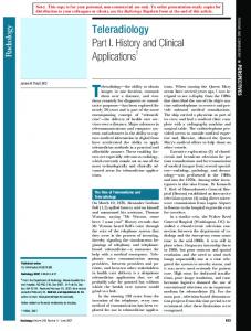
The model we use is composed of a water layer with a wavespeed of 1500 m/s. A flat, horizontal interface was placed at 2500 m depth. The contrast at the interface is produced by a velocity step from 1500 to 2200 m/s, with a constant background density of 1000 kg/m3 . The receivers were positioned in a horizontal line at 750 m depth, starting at lateral position x = 1500 m and ending at 3000 m, with increments of 25 m. The source line was also horizontal at a depth of 400 m, ranging from x = 500 m to 4500 m, with increments of 50 m. The data was modeled by 2D acoustic finitedifferencing with absorbing boundary conditions. Figure 5 shows that the data consists of direct and single-

reflected waves. As in the previous Section, we refer to these waves as u0 (rA,B , s) and uS (rA,B , s), respectively. First, we use the data in Figure 5 to analyze the integrands in equations 3 and 10. The deconvolution of the wavefield in Figure 5a with the wavefield in Figure 5b yields Figure 6a, while the cross-correlation yields Figure 6c. The deconvolution gather (Figure 6a) displays 2 2 causal term DAB , while both causal (CAB ) and acausal 3 (CAB ) contributions are present in the cross-correlation gather (Figure 6c). This confirms our claim that deconvolution interferometry gives mostly causal scattering 4 contributions (see Section 2.2.1). The term CAB also does not have a corresponding term in the deconvolution gather, as was predicted by equation 15. Also, the waveforms in Figure 6a are sharper than those in Figure 6c because deconvolution suppresses the source function. We use a water-level regularization method to do deconvolutions. For a brief discussion on this method see Appendix A in Vasconcelos and Snieder (2007b). The arrival times predicted with perturbation theory (bottom plots in Figure 6) provide an accurate representation of the modeled results in the top panels of Figure 6. In particular, the deconvolution series (equation 18, Figure 6b) describes well the most prominent terms in deconvolution interferometry (equation 10, Fig2 ure 6a). As predicted by theory, the terms DAB and 3 DAB have opposite polarity. The extrema of the curves in Figure 6 are stationary source positions. Thus, the stationary traveltime of each term is the time associated to the extremum of its curve in Figure 6. The sta1 1 tionary traveltimes from DAB and CAB are t = ±1 s, 2 representing causal and acausal direct waves. DAB and 2 CAB result in a stationary time of approximately 2.5 s, which coincides with the traveltime of a causal singlescattered wave. In previous Sections we showed that the 3 2 only coand DAB stationary traveltimes given by DAB incide when rA = rB . Since in Figure 6 rA 6= rB , the 3 2 stationary time of DAB is different from that of DAB . There are other events present in the lower lefthand corner of Figure 6a which are not present in Figure 6b. These events are described by higher-order terms of the deconvolution series (equation 18). Figure 7 shows how the events are described by terms of second and third order in the scattered wavefield. The events corresponding to third-order terms have considerably smaller amplitude than the ones related to second-order terms. Second-order terms are in turn weaker than the leadingorder terms (Figure 6a). A decrease in the power of the events with increasing order in the perturbed wavefield is expected, given the form of equation 18. These examples confirm the accuracy of the deconvolution series in describing the character of the integrand in deconvolution interferometry (equation 10). The integration over sources (e.g., equations 3 and 10) corresponds to the horizontal stack of the plots in Figures 6a and c. Stacking, for example, Figure 6c results in a single trace that represents a wavefield ex-


1500

-4

offset (m) 500 1000

1500

-4

-2 time (s)

time (s)

-2

0

0

2

0

2

4

0

offset (m) 500 1000

1500

-2 time (s)

-4

offset (m) 500 1000

0

215

0

2

4

4

(a)

(b)

(c)

Figure 8. Pseudo-shot (interferometric) gathers with the shot positioned at the receiver at 1500 m. The gather in (a) is obtained by deconvolution before stacking (equation 10), (b) is generated by cross-correlations (equation 3) and (c) is given by deconvolution after summation over sources (equation 24). Source integration of the gathers in Figures 6a and c yield the last trace in (a) and (b), respectively.

1

position (km) 2 3

4

0

position (km) 2 3

4

0

2 depth (km)

depth (km)

2

1

4

6

4

6

(a)

1

position (km) 2 3

4

2 depth (km)

0

4

6

(b)

(c)

Figure 9. Shot-profile wave-equation migrated images of the virtual shot gathers in Figure 8. In this figure, (a), (b) and (c) are the images obtained from migrating the gathers in Figure 8a, b and c, respectively. The true depth of the target interface is 2500 m. The shot is placed at 1.5 km and receivers cover a horizontal line from 1.5 to 3.0 km.

cited at a lateral position of 1500 m and recorded at 3000 m. We create an interferometric shot gather with a pseudo-shot placed at 1500 m by computing and stacking all of the deconvolution and cross-correlation gathers (Figures 6a and c) for the receiver fixed at 1500 m but varying the lateral position of the other receiver from 1500 to 3000 m. The interferometric shot gathers are shown in Figure 8. All gathers in Figure 8 show both causal and acausal direct waves. Only the gathers produced from cross-correlation (Figure 8b) and deconvolution after stack (Figure 8c) show causal and acausal reflections, agreeing with equations 3 and 28. The interferomet-

ric gather produced from deconvolution interferometry (Figure 8a) indeed only shows the causal scattered wave. 3 The first-order term DAB (equation 15) can be seen in Figure 8a with opposite polarity and slower moveout compared to the physical reflection. The reflection and 3 the DAB spurious events converge at zero-offset where they cancel. As observed in Figure 8a, this is due to the effect of the free point boundary condition (equation 16) imposed by the deconvolution of wavefields before source integration (see Section 2.2.1). As in Figure 8a, the zero-offset trace of the gather in Figure 8c consists of a band-limited spike at 0 s. This can be verified by setting CAB = CBB in equation 24. In contrast

216


to Figure 8a, Figure 8c does not contain the spurious events produced by the free point boundary condition present when deconvolving the wavefields before source integration. There are other events which are related to the truncated source integration (see Section 2.1). These are, for example, the upward-sloping linear events appearing between the direct arrivals and the reflections in all three gathers. The images obtained by shot-profile migration of the gathers in Figure 8 are shown in Figure 9. The shotprofile migration was done by wavefield extrapolation, with a split-step Fourier extrapolator. The reflector is placed at the correct depth in all three images. Also, all three images are remarkably similar, despite the differences between the gathers in Figure 8. The similarity between the images comes from the fact that the spurious events in deconvolution interferometry have a negligible effect in images made from offset-dependent data. Based on Figure 4, we argue in Section 2.4 that the spurious events produced by deconvolution interferometry typically do not map onto coherent reflectors. This justifies the absence of spurious reflectors in Figure 9a. In Figure 9, we can also appreciate the effect of deconvolution (Figures 9a and c) in compressing the waveform relative to cross-correlation (Figure 9b).

4

DISCUSSION AND CONCLUSIONS

By representing recorded wavefields as a superposition of direct and scattered wavefields, we derived a series expansion yielding terms that follow from performing deconvolution interferometry on receiver gathers before summing over sources. This derivation suggests that interferometry by deconvolution before stacking over sources gives only the causal scattered wavefield as if one of the receivers acted as a source. Because deconvolution interferometry requires the zero-offset wavefield to be zero at nonzero times, it generates spurious events to cancel scattered arrivals at zero-offset. We refer to this condition as the free point boundary condition at the pseudo-source location. With a simple model we illustrate this by using asymptotic approximations to the terms in deconvolution interferometry using the stationary-phase method. We also argue that interferometry can also be accomplished by deconvolution after summation over sources, which would yield terms analogous to correlation-based interferometry. Numerical examples with impulsive source data showed that deconvolution interferometry can successfully retrieve the causal response between two receivers. This response can be used to build interferometric shot gathers which in turn can be imaged. Imaging of deconvolution interferometric shot gathers proved to practically eliminate the spurious arrival generated by the deconvolution method. Indeed, our numerical asymptotic analysis suggests that the deconvolution-related spurious events add destructively in the imaging of offset-

variable data. It may be possible to create a reverse-time imaging scheme that results in an image free of spurious artifacts. We believe this could be done from the proper manipulation of boundary conditions in numerical modeling by the finite-difference method (Biondi, 2006). Although our assessment of the spurious events is model dependent, we believe that our observations also hold for more complicated models (see Part II of this article). Ideally, we want interferometry to give us the best possible representation of the impulse response between two given receivers. Cross-correlation interferometry yields an accurate representation of the waves propagating between the receivers, but it requires an estimate of the power spectrum of the wavelet for it to give an impulsive response. Deconvolution interferometry yields an impulsive response, but it does so at the cost of generating artifacts. Another option is to design an inverse filter to do interferometry (Sheiman, personal communication, 2006). For example, the inverse filter may require the zero-offset trace in the pseudo-shot with a pre-determined band-limited pulse. This inverse filter does not require any knowledge about the model, and its output would be described the deconvolution series discussed here. If there is some knowledge about the model, the inverse filter may be designed to replicate an estimate of a desired wavefield (e.g., Amundsen, 2001). In this case, the output of the inverse filter will approximate an impulsive version of cross-correlation interferometry. We associate the form of the deconvolution interferometry series to that of scattering series such as the Lippman-Schwinger series (Rodberg et al., 1967; Weglein et al. 2003). Forward and inverse scattering series serve, for instance, as the basis to methodologies in imaging and multiple suppression (Weglein et al., 2003). In analogy to scattering-based approaches, it is possible to express the deconvolution interferometry series in forward and inverse forms as well. Hence, an inverse deconvolution interferometry series may be designed for the imaging of pseudo-shots generated by deconvolution interferometry. The results we present here are consistent with previous deconvolution interferometry results. Although there is no explicit source integration in the work of Snieder and S ¸ afak (2006) and of Mehta et al. (2007a), their results agree with our representation of deconvolution interferometry before integration over sources. In the 1D models, such as used by Snieder and S ¸ afak (2006) and Mehta et al. (2007a), the excitation produced by teleseismic events was naturally in the stationary path between the receivers. This excludes the need for a full 3D source integration as in equation 10. Moreover, we argue that the application commonly referred to as receiver function (e.g., Shen et al. 1998, Mehta et al., 2007b) in global seismology is a direct application of deconvolution interferometry. With the same type of 1D layered model as in Snieder and S ¸ afak (2006) and of

Interferometry by deconvolution, Part I Mehta et al. (2007a), the receiver functions consist on the deconvolution of a radial receiver component with the vertical component of the same receiver. This, in interferometry terms, yields a zero-offset trace that corresponds to an excitation in the vertical direction whose wavefield is recorded in the radial direction. Also, like in Snieder and S ¸ afak (2006) and Mehta et al. (2007a), no source integration is required because in the 1D model all incoming waves are in the stationary wave-path. It is important to point out other perhaps less obvious relationships between our work and that of other authors. With an elegant derivation and examples, Loewenthal and Robinson (2000) show that deconvolutions between measured dual wavefields (e.g., particle velocity and pressure) can be used for modelindependent redatuming and for recovering reflectivity. Their derivation, in fact, is a proof of the application of deconvolution interferometry for dual wavefields. Amundsen (2001) designs deconvolution-type inverse operators to strip the influence of the water layer in marine data, at the same time performing free-surface multiple attenuation and estimating reflectivity. In a companion paper, Holvik and Amundsen (2005) use representation theorems of the same type as discussed in Section 2.1 along with deconvolution for elastic wavefield decomposition and multiple elimination. These papers are intimately related to deconvolution interferometry as we propose it. We advocate that the proper choice and manipulation of the wavefield pair u0 and uS give rise to different applications, with the example of dual wavefields by Loewenthal and Robinson (2001) or the boundary-condition approach by Amundsen (2001) and Holvik and Amundsen (2005). We also use these examples to highlight the potential of deconvolution-based interferometry in recovering data with amplitudes consistent with the subsurface reflectivity function. There are other important potential applications for deconvolution interferometry. As we summarized in Figure 1, deconvolution interferometry gives only causal wavefield perturbations, while unperturbed waves are present at both positive and negative times. For an ideal source coverage, the subtraction of the acausal wavefield from deconvolution interferometry from its causal response results only in wavefield perturbations. This idea may be useful for processing data from time-lapse experiments, as well as for pre-processing procedures such as direct- or surface-wave suppression. In the context of imaging, we highlight that in the cross-correlation imaging condition (Claerbout, 1985; Sava, 2006), the correlation serves the purpose of reproducing a zero-offset pseudo-shot experiment placed on top of a reflector (after extrapolating data to the reflector position). This is a direct application of the concept of correlation interferometry (e.g., Wapenaar and Fokkema). We believe that deconvolution interferometry can also be used to impose deconvolution imaging conditions (e.g., Muijs et al., 2007) that help to construct images whose ampli-

217

tudes are an estimate of subsurface reflectivity (Bleistein et al., 2001). Our goal here was to demonstrate the feasibility of using deconvolutions to recover the impulse response between receivers. Nonetheless, deconvolution interferometry has proven to be an important tool for interferometric imaging from complicated excitation. The Earth itself may be the cause of complicated source functions, as in the case of Snieder and S ¸ afak (2006) and of Mehta et al. (2007a). When using internal multiples for imaging, Vasconcelos et al. (2007b) found deconvolution interferometry to be necessary. In other applications the complicated character of the excitation may be related to the source itself. One such example is drill-bit seismology. When independent measures of the drill-bit stem noise are not available, deconvolution interferometry is necessary. This is the focus of the next part of this manuscript (Vasconcelos and Snieder, 2007b). Here, we highlight the physical differences between three interferometric methods: 1) deconvolution before source integration, 2) cross-correlations and 3) deconvolution after source integration. The comparison between methods 1) and 2) serves the purpose of providing the reader with information that allows one to relate the new content in this manuscript to much of the existing literature about interferometry. The understanding of the methods 2) and 3) provides the basis for the discussion about the specific use of deconvolution interferometry in drillbit seismic imaging, which is the subject of the second part of our study (Vasconcelos and Snieder, 2007b).

5

ACKNOWLEDGEMENTS

We thank the NSF (grant EAS-0609595) and the sponsors of the consortium for Seismic Inverse Methods for Complex Structures for their financial support. We are grateful to Kurang Mehta (CWP), Rodney Calvert and Jon Sheiman (both Shell) for insightful discussions and suggestions throughout this project. I.V. thanks Art Weglein for a private lecture on the inverse scattering series that inspired many of the ideas in this paper.

REFERENCES L. Amundsen. Elimination of free-surface related multiples without need of the source wavelet. Geophysics, 66:327341, 2001. A. Bakulin and R. Calvert. The virtual source method: Theory and case study. Geophysics, 71:SI139-SI150, 2006. A.J. Berkhout and D.J. Verschuur. Imaging of multiple reflections. Geophysics, 71:SI209-SI220, 2006. B. Biondi. 3D Seismic Imaging. Investigations in Geophysics, 14, Society of Exploration Geophysicists, 240 pages, 2006. N. Bleistein and R.A. Handelsman. Asymptotic expansions of integrals. Dover, New York, 1975.

218


N. Bleistein, J.K. Cohen and. J.W. Stockwell Jr. Mathematics of Multidimensional Seismic Imaging, Migration, and Inversion. Springer, New York, 2001. J.F. Claerbout. Synthesis of a layered medium from its acoustic transmission response. Geophysics, 33:264–269, 1968. J.F. Claerbout. Imaging the Earth’s Interior. Balckwell Publishing, 1985. A. Curtis, P. Gerstoft, H. Sato, R. Snieder and K. Wapenaar. Seismic interferometry - turning noise into signal. The Leading Edge, 25:1082–1092, 2006. D. Draganov, K. Wapenaar and J. Thorbecke. Seismic interferometry: Reconstructing the earths reflection response. Geophysics, 71:SI61-SI70, 2006. M. Fink. Time-reversal acoustics in complex environments. Geophysics, 71:SI151-SI164, 2006. E. Holvik and L. Amundsen. Elimination of the overburden response from multicomponent source and receiver seismic data, with source designature and decomposition into PP-, PS-, SP-, and SS-wave responses. Geophysics, 70:S43-S59, 2005. V. Korneev and A. Bakulin. On the fundamentals of the virtual source method. Geophysics, 71:A13-A17, 2006. D. Halliday, A. Curtis, D. van Mannen and J. Robertsson. Interferometric surface wave (ground roll) isolation and removal. submitted to Geophysics, 2007. E. Larose, L. Margerin, A. Derode, B. van Tiggelen, M. Campillo, N. Shapiro, A. Paul, L. Stehly and M. Tanter. Correlation of random wavefields: An interdisciplinary review. Geophysics, 71:SI11-SI21, 2006. O.I. Lobkis and R.L. Weaver. On the emergence of the Green’s function in the correlations of a diffuse field. J. Acoust. Soc. Am., 110:3011-3017, 2001. D. Loewenthal and E.A. Robinson. On unified dual wavefields and Einstein deconvolution. Geophysics, 65:293– 303, 2000. A. Malcolm, J. Scales and B.A. van Tiggelen. Extracting the Greens function from diffuse, equipartitioned waves. Physical Review E, 70:015601, 2004. D. van Manen, A. Curtis, and J.O.A. Robertsson. Interferometric modeling of wave propagation in inhomogeneous elastic media using time reversal and reciprocity. Geophysics, 71:SI47-SI60, 2006. K. Mehta, R. Snieder, R. Calvert and J. Sheiman. Virtual source gathers and attenuation of free-surface multiples using OBC data:implementation issues and a case study. Soc. Explor. Geophys. Expand. Abs., 2669–2673, 2006. K. Mehta, R. Snieder and V. Graizer. Extraction of nearsurface properties for a lossy layered medium using the propagator matrix. Geophys. J. Intl., in press, 2007. K. Mehta, R. Snieder and V. Graizer. Down-hole receiver function: a case study. Bull. Seism. Soc. Am., submitted, 2007. R. Muijs, J.O.A. Robertsson and K. Holliger. Prestack depth migration of primary and surface-related multiple reflections: Part I Imaging. Geophysics, 72:S59-SI69, 2006. H. Ohanian and R. Ruffini. Gr avitation and Spacetime. Norton & Co.,New York, 2nd Edition, 1994. F. Poletto and F. Miranda. Seismic while drilling, fundamentals of drill-bit seismic for exploration. Handbook of Geophysical Exploration, Vol 35, 2004. J.W. Rector III and B.P. Marion. The use of drill-bit energy as a downhole seismic source. Geophysics, 56:628-634, 1991.

J.E. Rickett and J.F. Claerbout. Acoustic daylight imaging via spectral factorization; helioseismology and reservoir monitoring. The Leading Edge, 19:957–960, 1999. L.S. Rodberg and R.M. Thaler. Introduction to the Quantum Theory of Scattering. Academic Press, New York, 1967. K.G. Sabra, P. Roux and W.A. Kuperman . Arrivaltime structure of the time-averaged ambient noise crosscorrelation function in an oceanic waveguide. J. Acoust. Soc. Am., 117:164–174, 2004. K.G. Sabra, P. Gerstoft, P. Roux, W.A. Kuperman and M. Fehler. Surface-wave tomography from microseisms in Southern California. Geophys. Res. Let., 32:L14311, 2005. P. Sava. Time-shift imaging condition in seismic migration. Geophysics, 71:S209–S217, 2006. G.T. Schuster, F. Followill, L.J. Katz, J. Yu, and Z. Liu. Autocorrelogram migration: Theory. Geophysics, 68:16851694, 2004. G.T. Schuster and M. Zhou. A theoretical overview of modelbased and correlation-based redatuming methods. Geophysics, 71:SI103-SI110, 2006. N.M. Shapiro, M. Campillo, L. Stehly, and M.H. Ritzwoller. High-resolution surface-wave tomography from ambient seismic noise. Science, 307:1615-1618, 2005. Y. Shen, A.F. Sheehan, K.G. Dueker, C. de Groot-Hedlin and H. Gilbert. Mantle Discontinuity Structure Beneath the Southern East Pacific Rise from P-to-S Converted Phases. Science, 280:1232–1235, 1998. R. Snieder. Extracting the Green’s function from the correlation of coda waves: A derivation based on stationary phase. Phys. Rev. E., 69:046610, 2004. R. Snieder and E. S ¸ afak. Extracting the building response using seismic interferometry; theory and application to the Millikan library in Pasadena, California. Bull. Seismol. Soc. Am., 96:586-598, 2006. R. Snieder, K. Wapenaar and K. Larner. Spurious multiples in seismic interferometry of primaries. Geophysics, 71:SI111-SI124, 2006a. R. Snieder, J. Sheiman and R. Calvert. Equivalence of the virtual-source method and wave-field deconvolution in seismic interferometry. Phys. Rev. E, 73:066620, 2006b. R. Snieder. Retrieving the Greens function of the diffusion equation from the response to a random forcing. Phys. Rev. E, 74:046620, 2006. R. Snieder. Extracting the Greens function of attenuating heterogeneous acoustic media from uncorrelated waves. J. Acoust. Soc. Am., in press, 2007. R. Snieder, K. Wapenaar, and U. Wegler. Unified Green’s function retrieval by cross-correlation; connection with energy principles. Phys. Rev. E, 75:036103, 2007. J. Trampert, M. Cara and M. Frogneux. SH propagator matrix and Qs estimates from borehole- and surfacerecorded earthquake data. Geophys. J. Intl., 112:290– 299, 1993. I. Vasconcelos and R. Snieder. On representation theorems and seismic interferometry in perturbed media. Geophysics, in preparation, 2007a. I. Vasconcelos and R. Snieder. Interferometry by deconvolution, Part II: application to drill-bit seismic imaging. Geophysics, in preparation, 2007b. I. Vasconcelos, R. Snieder, S.T. Taylor, P. Sava, J.A. Chavarria and P. Malin. High Resolution Imaging of the San Andreas Fault at Depth. Science, in preparation, 2007a.

Interferometry by deconvolution, Part I I. Vasconcelos, R. Snieder and B. Hornby. Imaging with internal multiples from subsalt VSP data: examples of controlled illumination in interferometry experiments. Geophysics, in preparation, 2007b. K. Wapenaar. Retrieving the elastodynamic Green’s function of an arbitrary inhomogeneous medium by cross correlation. Phys. Rev. Lett., 93:254301, 2004. K. Wapenaar, J. Thorbecke, and D. Dragonov. Relations between reflection and transmission responses of threedimensional inhomogeneous media. Geophys. J. Int., 156:179–194, 2004. K. Wapenaar. Green’s function retrieval by cross-correlation in case of one-sided illumination. Geophys. Res. Lett., 33:L19304, 2006. K. Wapenaar, E. Slob, and R. Snieder. Unified Green’s Function Retrieval by Cross Correlation. Phys. Rev. E., 97:234301, 2006. R.L. Weaver and O.I. Lobkis. Ultrasonics without a source: Thermal fluctuation correlations and MHz frequencies. Phys. Rev. Lett., 87:134301–1/4, 2001. R.L. Weaver and O.I. Lobkis. Diffuse fields in open systems and the emergence of the Green’s function. J. Acoust. Soc. Am., 116:2731–2734, 2004. A.B. Weglein, F.V. Ara´ ujo, P.M. Carvalho, R.H. Stolt, K.H. Matson, R.T. Coates, D. Corrigan, D.J. Foster, S.A. Shaw, and H. Zhang. Inverse scattering series and seismic exploration. Inverse Problems, 19:R27–R83, 2003. K. van Wijk. On estimating the impulse response between receivers in a controlled ultrasonic experiment. Geophysics, 71:SI79-SI84, 2006. J. Yu and G.T. Schuster. Crosscorrelogram migration of inverse vertical seismic profile data. Geophysics, 71:S1-S11, 2006.

219

220


APPENDIX A: PHYSICAL ANALYSIS OF THE DECONVOLUTION INTERFEROMETRY SERIES According to the derivation in Section 2.2.1, the deconvolution in equation 9 can be expressed in series form

DAB

«n ∞ „ X CAB GS (rB , s) G∗S (rB , s) = − − ∗ . G0 (rB , s) G0 (rB , s) |G0 (rB , s)|2 n=0

(A1)

The objective of this appendix is to reproduce the steps and physical approximations that simplify the series in equation A1. Let us first consider the n = 2 term in the summation in equation A1, which is „

S2 =

G∗ (rB , s) GS (rB , s) − S∗ − G0 (rB , s) G0 (rB , s)

«2

(A2)

Substituting this term in the expansion of |G(rB , s)|−2 (equation 13) gives, to second order in GS , |G(rB , s)|−2

≈

– G∗ (rB , s) GS (rB , s) − S∗ G0 (rB , s) G0 (rB , s) "„ # «2 „ ∗ «2 1 GS (rB , s) GS (rB , s) |GS (rB , s)|2 + , + + 2 G0 (rB , s) G∗0 (rB , s) |G0 (rB , s)|2 |G0 (rB , s)|2 1 |G0 (rB , s)|2

»

1−

(A3) 2

2

where the very last term is zero-phase. When |G0 | >> |GS | , the zero-phase term in equation A3 can be neglected because it does not contribute with any new arrival. Equation A3 thus simplifies to

|G(rB , s)|−2 ≈

1 |G0 (rB , s)|2

"

GS (rB , s) G∗ (rB , s) − S∗ + G0 (rB , s) G0 (rB , s)

1−

„

GS (rB , s) G0 (rB , s)

«2

+

„

G∗S (rB , s) G∗0 (rB , s)

«2 #

;

(A4)

for which the actual contribution from n = 2 to the sum in equation A1 is „

S2 ≈

uS (rB , s) u0 (rB , s)

«2

+

„

u∗S (rB , s) u∗0 (rB , s)

«2

,

(A5)

instead of the full S2 term in equation A2. Applying the same rationale for the simplification of S2 to the n = 3 term from the summation in equation A1 gives

S3 =

„

−

GS (rB , s) G∗ (rB , s) − S∗ G0 (rB , s) G0 (rB , s)

«3

.

(A6)

S3 can be expressed in terms of S2 , such that S3 = S2 ×

„

−

G∗ (rB , s) GS (rB , s) − S∗ G0 (rB , s) G0 (rB , s)

«

.

(A7)

Using the simplified S2 (equation A5) in evaluating S3 gives „

«3

„

«3

|GS (rB , s)|2 G∗S (rB , s)G0 (rB , s) |GS (rB , s)|2 GS (rB , s)G∗0 (rB , s) − 2 2 |G0 (rB , s)| |G0 (rB , s)| |G0 (rB , s)|2 |G0 (rB , s)|2 (A8) The last two terms of S3 in the above equation are not zero-phase. Note also that despite` being nonzero phase, the ´ phase of these terms is the same of other terms of lower order. For example, the term |GS |2 / |G0 |4 GS G∗0 has 2 the same phase as the integrand in the DAB term in equation 15, but with weaker amplitude and opposite polarity. Because they do not result in new arrivals and have weak amplitudes, we drop the last two terms in equation A8 and reduce S3 to S3 ≈ −

GS (rB , s) G0 (rB , s)

−

G∗S (rB , s) G∗0 (rB , s)

−

S3 ≈ −

„

GS (rB , s) G0 (rB , s)


221

«3

(A9)

−

„

G∗S (rB , s) G∗0 (rB , s)

«3

.

Any Sn term of the summation in equation A1 can be written in terms of Sn−1 in the same form of equation A7. Analogously to equation A8, any Sn will yield four terms from which two terms can be dropped according to the same rationale we use to neglect the last two terms in equation A8. Thus, by induction, the summation in equation A1 simplifies to ∞ „ X

n=0

G∗ (rB , s) GS (rB , s) − S∗ − G0 (rB , s) G0 (rB , s)

«n

≈ 1+

∞ X

(−1)

n

n=1

»„

GS (rB , s) G0 (rB , s)

«n

+

„

G∗S (rB , s) G∗0 (rB , s)

«n –

.

(A10)

Using this simplified summation in the deconvolution series gives

DAB

CAB ≈ |G0 (rB , s)|2

1+

∞ X

(−1)

n

n=1

»„

GS (rB , s) G0 (rB , s)

«n

+

„

G∗S (rB , s) G∗0 (rB , s)

«n –!

.

(A11)

The term-by-term expansion of the equation above is such that for any given value of n, the terms

DAB,terms = (−1)n

„

G∗S (rB , s) G∗0 (rB , s)

cancel, for n + 1, with the terms

DAB,terms = (−1)n+1

„

G∗S (rB , s) G∗0 (rB , s)

«n

1

0

C B BG0 (rA , s)G∗S (rB , s) + GS (rA , s)G∗S (rB , s)C @| {z } {z }A |

«n+1

2 CAB

1

0

C B BG0 (rA , s)G∗0 (rB , s) + GS (rA , s)G∗0 (rB , s)C ; @| {z } {z }A | 1 CAB

(A12)

4 CAB

(A13)

3 CAB

which in the limit n → ∞ leaves only the contribution of the causal ratio GS /G0 to DAB in equation A11. The cancelation of the terms proportional to the acausal ratio G∗S /G∗0 (highlighted by equations A12 and A13) is responsible 3 4 for the absence of acausal terms having the same phase as CAB and CAB (equation 4) in deconvolution interferometry (equation 15). Because of these successive cancelations, we arrive to

DAB ≈

„ «n ∞ X G0 (rA , s)G∗0 (rB , s) GS (rB , s) GS (rA , s)G∗0 (rB , s) CAB n (−1) + + , G0 (rB , s) |G0 (rB , s)|2 |G0 (rB , s)|2 |G0 (rB , s)|2 n=1

(A14)

«n „ ∞ X CAB G(rA , s) GS (rB , s) n + . (−1) G0 (rB , s) G0 (rB , s) |G0 (rB , s)|2 n=1

(A15)

which, in compact form, gives

DAB ≈

We present this approximate deconvolution series as a tool to identify the most prominent events within the integrand of the deconvolution interferometry integral (equation 10). Equation A14 is also useful in the description of the kinematics of deconvolution interferometry terms, as we discuss in the main text. If one seeks to describe the result of deconvolution interferometry with a more accurate dynamic behavior, the original series in equation A1 is more appropriate.

222


APPENDIX B: STATIONARY-PHASE EVALUATION OF LEADING ORDER TERMS The wavefields shown in Figure 3 can be described by the ray-geometric impulse responses u0 (rA,B , s)

| | , and |rA,B − s|

ik rA,B − s

= G0 (rA,B , s) = − e4π

(B1) uS (rA,B , s)

= GS (rA,B , s) =

ik

(|rsr

−r

| + |s − rsr |)

A,B A,B A,B e −r 4π − rA,B | + |s − rsr (|rsr A,B A,B |)

;

where rsr A,B are the specular reflection points for the receiver-source pairs (rA,B , s). G0 and GS are the far-field acoustic Green’s functions we use to describe u0 and uS , respectively. In our model, s = (x, y, z = 0) and rA,B = (xA,B , yA,B = 0, zA,B ). The distances in the phases and denominators in equation B1 can be expressed in terms of 1 the corresponding ray-lengths in Figure 3. Using the Green’s functions in equation B1 to express DAB (equation 15) we get Z ik(LA −LB ) 1 e dxdy , (B2) 2 LA LB (4πLB ) where ϕ = ik (LA − LB ) is the phase of the integrand. The source position that gives a stationary contribution to the integral in equation B2 satisfies 1 DAB =

y y ∂ϕ − ; = ∂y LA LB

(B3)

∂ϕ x − xB x − xA − = sin ψA − sin ψB , = ∂x LA LB

(B4)

0= and 0=

where ψA and ψB is the angle defined between the direct wave and the vertical at receivers A and B. It follows from 1 equations B3 and B4 that the stationary point for the source in the DAB term satisfies (Snieder et al., 2006) ψA = ψB = ψ

and

y=0.

(B5)

It is expected that the stationary contribution for all terms comes from sources at y = 0 because yA,B = 0 and the model is a flat reflector in a homogeneous and isotropic medium. The condition ψA = ψB (equation B5) states that the stationary source is the one that sends a direct wave which is first recorded at rB and goes straight to rA . This 1 is the same stationary condition as for the CAB term of Snieder et al. (2006). To approximate the integral in equation B2 with the stationary-phase method we must evaluate, at the stationary point, the second derivatives ∂2ϕ ∂x2

=

2 z2 1 zA z2 z2 1 − B − B = A 3 3 2 LA LB LA LA L2B LB

= cos 2 ψ

„

1 1 − LA LB

«

(B6)

,

and 1 L2 L2 1 ∂2ϕ − . = 3A − B = 2 ∂y LA L3B LA LB

(B7)

Based on these second derivatives, the stationary-phase approximation (Bleistein and Handelsman, 1975) to equation B2 is


1 DAB

n 1 exp (ik (LA − LB )) = 2 LA LB (4πLB ) (4π)2

×e

×e

−iπ/4

−iπ/4

r r

2π s k

223

1 cos 2 ψ

„

1 1 − LB LA

1 2π r , k 1 1 − LB LA

«

(B8)

where k = ωc . At the stationary source point, where ψA = ψB , the distance LA − LB is equivalent to the distance 1 |rA − rB |. Thus, in the stationary-phase approximation, DAB is given by 1 DAB =

nc G0 (rA , rB ) . 32π 2 L2B cosψ (−iω)

(B9)

1 From the derivation above, the stationary-phase evaluation of DAB is completely analogous to the evaluation of 1 2 CAB (equation 4) in Snieder et al. (2006). Since the same occurs with the term DAB , we refrain from reproducing the steps of its stationary-phase approximation in this paper, and refer the readers to Snieder et al. (2006) for these steps.

224


Interferometry by deconvolution, Part I: Theory and ... - Semantic Scholar

Interferometry by deconvolution, Part I: Theory and ... - Semantic Scholar

Suggest Documents

Interferometry by deconvolution, Part 1â Theory ... - Semantic Scholar

Seismic interferometry using multidimensional deconvolution and

Universes in Type Theory Part I â Inaccessibles ... - Semantic Scholar

Seismic interferometry by crosscorrelation and by ... - Semantic Scholar

Polar-interferometry - Semantic Scholar

Higher Spin Theory-Part I

Microcanonical multifractal formalism: Part I ... - Semantic Scholar

A Learning Machine: Part I - Semantic Scholar

Part I-September 2005.indd - Semantic Scholar

A Learning Machine: Part I - Semantic Scholar

Medical Imaging Part I - Semantic Scholar

for holographic interferometry - Semantic Scholar

Burst-mode and scanSAR interferometry - Semantic Scholar

Part I: The Theory of International Regimes

CONTENTS Part I: Linear Theory

Fine Arts Theory Part-I - NTI

Part I Type Theory & Equality Reflection - CIRM

Digital Instruments and Players: Part I â Efficiency ... - Semantic Scholar

Teleradiology Part I. History and Clinical Applications - Semantic Scholar

Revising Z: Part I - logic and semantics - Semantic Scholar

Triage in Medicine, Part I: Concept, History, and ... - Semantic Scholar

Practical bandwidth selection in deconvolution ... - Semantic Scholar

three-dimensional volumetric deconvolution - Semantic Scholar

SATELLITE IMAGE DECONVOLUTION USING ... - Semantic Scholar

Interferometry by deconvolution, Part I: Theory and ... - Semantic Scholar