HUNGARIAN JOURNAL OF INDUSTRIAL CHEMISTRY VESZPRÉM Vol. 35. pp. 101-108 (2007)
INTERPETABLE SUPPORT VECTOR MACHINES IN REGRESSION AND CLASSIFICATION – APPLICATION IN PROCESS ENGINEERING T. KENESEI, J. ABONYI University of Pannonia, Department of Process Engineering, H-8201 Veszprém, P.O.Box 158, HUNGARY
[email protected], www.fmt.vein.hu/softcomp
Tools from the armoury of soft computing have been in focus of researches recently, since soft computing techniques are used for fault detection (classification techniques), forecasting of time-series data, inference, hypothesis testing, and modelling of causal relationships (regression techniques) in process engineering. These techniques solve two cardinal problems: learning from experimental data by neural networks and support vector based techniques and embedding existing structured human knowledge into fuzzy models. Support vector based models are one of the most commonly used soft computing techniques. Support vector based models are strong in feature selection and to achieve robust models and fuzzy logic helps to improve the interpretability of models. This paper deals with combining these existing soft computing techniques to get interpretable but accurate models for industrial purposes. The paper describes that trained support vector based models can be used for the construction of fuzzy rule-based classifier or regression models. However, the transformed support vector model does not automatically result in an interpretable fuzzy model because the support vector model results in a complex rulebase, where the number of rules is approximately 40-60% of the number of the training data. Hence, reduction of the support model-initialized fuzzy model is an essential task. For this purpose, a three-step reduction algorithm is used on the combination of previously published model reduction techniques. In the first step, the identification of the SV model is followed by the application of the Reduced Set method to decrease the number of kernel functions. The reduced SV model is then transformed into a fuzzy rule-based model. The interpretability of a fuzzy model highly depends on the distribution of the membership functions. Hence, the second reduction step is achieved by merging similar fuzzy sets based on a similarity measure. Finally, in the third step, an orthogonal least-squares method is used to reduce the number of rules and re-estimate the consequent parameters of the fuzzy rule-based model. The proposed approach is applied for classification problems and applied for Hammerstein system identification to illustrate the effectiveness of the technique.
Introduction Tools from the armoury of soft computing have been in focus of researches recently, since soft computing techniques are used for fault detection (classification techniques), forecasting of time-series data, inference, hypothesis testing, and modelling of causal relationships (regression techniques) in process engineering. As mankind use, store and maintain enormous size of information in databases (the amount of data used doubles almost every year) modelling techniques getting more and more important. This phenomenon implies the need of new generation computational techniques to support knowledge extraction from data sources. Historically the notion of finding useful patterns in data has been given a variety of names including data mining, knowledge extraction, information discovery, and data pattern processing. The term data mining has been mostly used by statisticians, data analysts, and the management information systems (MIS) communities. [1]
The term knowledge discovery in databases (KDD) refers to the overall process of discovering knowledge from data, while data mining refers to a particular step of this process. Data mining is the application of specific algorithms for extracting patterns from data. The additional steps in the KDD process, such as data selection, data cleaning, incorporating appropriate prior knowledge, and proper interpretation of the results are essential to ensure that useful knowledge is derived form the data [2]. Soft computing techniques are one of the cornerstones of the KDD process. This paper gives a method how the techniques of soft computing can be combined to get interpretable and robust models for the KDD process. The meaning of soft computing was originally tailored in the early 1990s by Dr. Zadeh [3]. Soft computing refers to a collection of computational techniques in computer science, artificial intelligence, machine learning and some engineering disciplines, to solve two cardinal problems: ● Learning from experimental data (examples, samples, measurements, records, patterns) by
102 neural networks and support vector based techniques ● Embedding existing structured human knowledge (experience, expertise, heuristic) into fuzzy models [2] These approaches attempt to study, model, and analyze very complex phenomena: those for which more conventional methods have not yielded low cost, analytic, and complete solutions. Earlier computational approaches (hard computing) could model and precisely analyze only relatively simple systems. As more complex systems arising in biology, medicine, the humanities, management sciences, and similar fields often remained intractable to conventional mathematical and analytical methods. Where the hard computing schemes, which strive for exactness and full truth, fail to render the problem, soft computing techniques exploit the given tolerance of imprecision, partial truth, and uncertainty is inherent in human thinking and in real life problems, to deliver robust, efficient and optimal solutions and to further explore and capture the available design knowledge. Generally speaking, soft computing techniques resemble biological processes more closely than traditional techniques, which are largely based on formal logical systems, such as sentential logic and predicate logic, or rely heavily on computer-aided numerical analysis. Support vector based models and neural networks are one of the most commonly used soft computing techniques. However it should be pointed out that simplicity and complexity of these systems is a challenging task to perform. Neural networks, support vector machines are universal approximators of any multivariate function; they are widely-used to model highly nonlinear, unknown or partially known complex systems plants or processes. The identification of the proper structure of nonlinear neural networks (NNs) and Support Vector Based techniques (SVM, SVR) is a challenging task, since these black-box models are too complex and not interpretable. Complexity and interpretability issues are connected with each other: achieve the less complex more interpretable model with the best accuracy. Other problem is how a priori knowledge can be utilized and integrated into the black box modelling approach, and how a human expert can validate the identified black box model or more favourably, follow the identification process to interfere in it if it is needed (e.g. to avoid over parameterization) Neural Networks and Support Vector Machines are strong in feature selection and to achieve robust models and fuzzy logic helps to improve the interpretability of models. With the combination of these techniques accurate, but interpretable models can be achieved. This paper describes a three-step technique how to use reduction techniques on trained SVM and SVR models to acquire transparent, but accurate fuzzy rule based classifier and fuzzy regression models. The steps are the following:
Step 1. - Reduced Set method The identification of the SVM/SVR model is followed by the application of the Reduced Set (RS) method to decrease the number of kernel functions. Originally, this method has been introduced by [4] to reduce the computational complexity of SV models. Step 2. - Similarity-based fuzzy set merging The Gaussian membership functions of the fuzzy rulebased models are derived from the Gaussian kernel functions of the SV models. The interpretability of a fuzzy model highly depends on the distribution of the membership functions. Hence, the next reduction step is achieved by merging fuzzy sets based on a similarity measure. [5] Step3. - Rule-base simplification by orthogonal transformations Finally, an orthogonal least-squares method is used to reduce the number of rules and re-estimate the consequent parameters of the classifier. The application of orthogonal transforms for reducing the number of rules has received much attention in the recent literature [6, 7]. These methods evaluate the output contribution of the rules to obtain the order of importance. The less important rules are then removed according this ranking to further reduce the complexity and increase the transparency. This article organized as follows. Firstly basic notations of support vector machines and the connection between the fuzzy rule-based classifiers is described, later on the connection between support vector regression and fuzzy regression is introduced. After detailed description of the three-step reduction algorithm examples indicate the power and the usage of the described techniques either on classification and regression problems.
Support vector machines for classification Formulation of the fuzzy rule-based classifier as a kernel machine SVM has been recently introduced for solving pattern recognition and function estimation problems. SVM is a nonlinear generalization of the Generalized Portrait algorithm developed in Russia in the 1960s. In its present form, the SVM was developed at AT&T Bell Laboratories by Vapnik and co-workers.[8] Due to this industrial context, SVM research has up to date had a sound orientation towards real-world applications. SVM learning has now evolved into an active area of research. Moreover, it is in the process of entering the standard methods toolbox of machine learning. The basic idea behind SVM is that with a kernel function k(xi, xj) which for all data pairs {x1, ... xNd} ⊂ χ × RNi give rise to positive matrices Kij := k(xi, xj). [9] Using K instead of a dot product in RNi corresponds to mapping the data into a possibly high dimensional space F, by a
103 usually nonlinear map φ : RNi → F and takes the dot product there k(zi, x) = (φ(zi), φ (x))
(1)
are effective in solving nonlinear problems because they map the original input space into a nonlinear feature space by using membership functions similar to the SVM that utilizes kernel functions for this purpose.
The structure of the fuzzy rule-based classifier
Support vector machines for regression
One widely used approach to solve non-fuzzy Nc-class pattern recognition problems is to consider the general problem as a collection of binary classification problems. Accordingly, Nc classifiers can be constructed, i.e. one for each class. The c-th classifier, c = 1 ... Nc, separates class c from the Nc other classes. This one-against-all method results in a hierarchical classifier structure that allows for a sequential model construction and evaluation procedure. Based on this the classifier consist of Nc fuzzy subsystems with a set of Takagi-Sugeno-type fuzzy rules [10] that describe the c-th class in the given data set as:
SVMs can also be applied to regression problems as described in the following paragraphs. Suppose we have the training data {(x1, y1) ... (xNd, yNd)} ⊂ χ × RNi, where χ denotes the space of input patterns. Our goal is to find function f(x) that has at most ε deviation from the actually obtained targets yi for all the training data. In other words we do not care about errors as long as they are less than ε, but will not accept any deviation larger than this [9]. The linear case is the following:
c
Ri if x1 is Aic1 and ... xn is Ainc then yic = δ ic
(2)
c
where Ri is the i-th rule in the c-th fuzzy rule-based c classifier and NR denotes the number of rules. Aic1 , K ANc i
denote the antecedent fuzzy sets that define the operating region of rule in the Ni dimensional input space. The c rule consequent δi is a crisp number. The connective is modelled by the product operator. Hence the degree of activation of the i-th rule is calculated as Ni
β ic (x ) = ∏ Aijc (x j ), i = 1,K, N Rc
f (x ) = z, x + b with z ∈ χ , b ∈ R
Ni
1 z 2 ⎧ yi − z , xi − b ≤ ε s.t.⎨ ⎩ z , xi + b − yi ≤ ε
min
(7)
Sometimes however we want to allow some errors. This could be done by the introduction of an alternative loss function. The loss function must be modified to include a distance measure.
(3)
j =1
a
b
c
d
The output of the classifier determined by the following decision function ⎞ ⎛ N Rc y c = sgn ⎜ ∑ β ic ( x )δ ic + b c ⎟ ⎟ ⎜ i =1 ⎠ ⎝
(4)
where bc is a constant threshold. If yc = –1, then it is not an item in class c. The main principle of kernel-based support vector classifiers is the identification of a linear decision boundary in this high-dimensional feature-space. The link to the fuzzy model structure is the following: The fuzzy sets are represented in this paper by Gaussian membership functions
(
⎛ x j − z ij Aij x j = exp⎜ ⎜ 2σ 2 ⎝
( )
)
2
⎞ ⎟ ⎟ ⎠
⎛ x−z i β i (x ) = k ( zi , x) = exp⎜ ⎜ 2σ ⎝
(5) 2
⎞ ⎟ ⎟ ⎠
(6)
The degree of fulfilment βi(x) can be written in a more compact form by using the Gaussian kernels. This kernel interpretation of fuzzy systems shows that fuzzy models
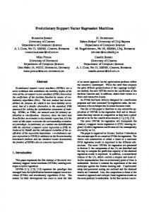
Figure 1: Loss functions The loss function in Fig. 1(a) corresponds to the conventional least squares error criterion. The loss function in Fig. 1(b) is a Laplacian loss function that is less sensitive to outliers than the quadratic loss function. Huber proposed the loss function in Fig. 1(c) as a robust loss function that has optimal properties when the underlying distribution of the data is unknown. These three loss functions will produce no sparseness in the support vectors. To address this issue Vapnik proposed the loss function, also called ε-insensitive loss function in Fig. 1(d) as an approximation to Huber’s loss function that enables a sparse set of support vectors to be obtained [11]. The nonlinear SVR problems with the ε-insensitive loss function (Fig. 1(d)) is given by:
104 ⎧ 1 Nd ∗ ∗ ⎪− ∑ (α i − α i )(α j − α j )k xi , x j ⎪ 2 i , j =1 maximize⎨ Nd Nd ⎪ − ε α +α ∗ + y α −α ∗ ∑ ∑ i i i i i ⎪⎩ i =1 i =1
(
(
)
(
)
∑ (α i − α ) = 0 i =1 α i ,α j ∈ [0, C ]
subject to and
Nd
procedure similar fuzzy sets are merged when their similarity exceeds a user-defined threshold θ ∈ [0, 1]. The set-similarity measure can be based on the settheoretic operations of intersection and union [12]:
)
∗ i
(8)
where α is the Lagrange multiplier (α* is the dual variable); the kernel function k; C > 0 represents the trade-off between the flatness of f and the deviation tolerance. We can rewrite the equation above to formulate the so called Support Vector expansion: Nd
(
(
)
S Aij , Akj =
∗
(
)
S Aij , Akj =
)
Nd
i =1
(
)
The link between support vector based techniques and fuzzy models is established in the earlier sections through equations 1-6. To get a fuzzy-rule based regression model from the support vector regression model the following interpretation is needed: NR
(
)
(z
1
ij
− z kj
) + (σ 2
ij
− σ kj
(12)
)
2
(9)
Formulation of the fuzzy regression model based on support vector regression
y = ∑ β i (x )δ i + b
1 = 1 + d Aij , Akj 1+
Reduction of the number of rules by orthogonal transforms
where z = ∑ α i − α ∗i φ (xi )
(11)
Aij ∪ Akj
where |·| denotes the cardinality of a set, and the ∩ and ∪ operators represent the intersection and union, respectively, or it can be based on the distance of the two fuzzy sets. Here, the following expression was used to approximate the similarity between two Gaussian fuzzy sets [13]:
f ( x) = ∑ α i − α i k (xi , x ) + b i =1
Aij ∩ Akj
(10)
i =1
where βi is the firing strength and δi is the rule consequent. Reduction of the number of fuzzy sets
In the previous section, it has been shown how kernelbased models with a given number of kernel functions NR, can be obtained. Because the number of the rules in the transformed fuzzy system is identical to the number of kernels, it is extremely important to get a moderate number of kernels in order to obtain a compact fuzzy rule-based model. From (6) it can be seen that the number of fuzzy sets in the identified model is Ns = NR · Ni. The interpretability of a fuzzy model highly depends on the distribution of these membership functions. With the simple use of (6), some of the membership functions may appear almost undistinguishable. Merging similar fuzzy sets reduces the number of linguistic terms used in the model and thereby increases the transparency of the model. This reduction is achieved by a rule-base simplification method [12, 13], based on a similarity measure S(Aij, Akj), i, k, = 1, ..., n; and i≠j. If S(Aij, Akj) = 1, then the two membership functions Aij and Akj are equal. S(Aij, Akj) becomes 0 when the membership functions are non-overlapping. During the rule-base simplification
By using the previously presented SV model identification and reduction techniques, the following fuzzy rule-based models have been identified. For classification:
(
⎛ N R Ni ⎛ x j − z ij y = sgn ⎜ ∑∏ exp⎜ ⎜ i =1 j =1 ⎜ 2σ 2 ⎝ ⎝
)
2
⎞ ⎞ ⎟δ + b ⎟ i ⎟ ⎟ ⎠ ⎠
(13)
For regression:
(
N R Ni ⎛ x j − zij y = ∑∏ exp⎜ ⎜ 2σ 2 i =1 j =1 ⎝
)
2
⎞ ⎟δ + b ⎟ i ⎠
(14)
Because the application of the RS method and the fuzzy set merging procedure the obtained membership functions only approximate the original feature space identified by the SV based model. Hence, the δ = [δ1, δ2, ..., δNR]T consequent parameters of the rules have to be re-identified to minimize the difference between the decision function of the support vector machine and the fuzzy model (13, 14): 2
NR ⎛ Ni ⎞ MSE = ∑ ⎜⎜ ∑ γ i k x j , xi − ∑ δ i β i x j ⎟⎟ = y s − Bδ i =1 j =1 ⎝ i =1 ⎠ Nd
(
)
( )
2
(15)
where the matrix B = [b1 , K , b NR ] ∈ R Nd ×N R containing the firing strength of all NR rules for all the input xi, where bj = [βj(x1), ..., βj(xNd)]T. As the fuzzy rule-based model (13, 14) is linear in the parameters δ, (15) can be solved by a least-squares method δ = B+ ys +
(16)
where B denotes the Moore-Penrose pseudo inverse of B. The application of orthogonal transforms for the above mentioned regression problem (15) for reducing the number of rules has received much attention in recent literature [14]. These methods evaluate the output contribution of the rules to obtain an importance ordering. For modelling purposes, the Orthogonal Least Squares
105 (OLS) is the most appropriate tool [7]. The OLS method transforms the columns of B into a set of orthogonal basis vectors in order to inspect the individual contribution of each rule. To do this, Gram-Schmidt orthogonalization of B = WA is used, where W is an orthogonal matrix WT W = I and A is an upper triangular matrix with unity diagonal elements. If wi denotes the i-th column of W and gi is the corresponding element of the OLS solution vector g = Aδ, the output variance ysT y/Nd can be explained by the regressors
Nr
∑ g i w Ti w i / N d . Thus, the i =1
error reduction ratio, ρ, due to an individual rule i can be expressed as
ρi =
g u2 wiT wi y sT y s
This model has been reduced by the RS method, by which we tried to reduce the model by a factor of 10, NR = 8. By this step, the classification performance slightly decreased on the training set to 12 misclassifications, but the validation data showed a slightly better result with 14 misclassifications. Next, the reduced kernelclassifier was transformed into a fuzzy system. Fig. 2 shows the membership functions that were obtained. The obtained model with eight rules is still not really well interpretable; however, some of the membership functions appear very similar and can probably be merged easily without loss in accuracy.
(17)
This ratio offers a simple mean for ordering the rules, and can be easily used to select a subset of rules in a forward-regression manner. Evaluating only the approximation capabilities of the rules, the OLS method often assigns high importance to a set of redundant or correlated rules. To avoid this, in [7] some extension for the OLS method were proposed. In the previous sections it has been shown how an SV based model, that is structurally equivalent to a fuzzy model, can be identified. Unfortunately, this identification method cannot be used directly for the identification of interpretable fuzzy systems because the number of the support vectors is usually very large. Typical values are 40-60% of the number of training data which is in our approach equal to the number of rules in the fuzzy system. Therefore, there is a need for an interpretable approximation of the support vector expansion. For this purpose the three-step algorithm described will be used in the Examples section
Figure 2: Non-distinguishable membership functions obtained after the application of the RS method
Examples Example for classification To show the power of the described technique is applied to the Wisconsin Breast Cancer data, which is a benchmark problem in the classification and pattern recognition literature. The data is divided into training and an evaluation subset that have similar size and class distributions (We used 342 cases for training and 341 cases for testing the classifier). First, the advanced version of C4.5 was applied to obtain an estimate for the useful features. This method gave 36 misclassification for the problem (5,25 %). The constructed decision-tree model had 25 nodes and used mainly three inputs; x1, x2 and x6. Based on this pre-study, only the previous three inputs were applied to identify the SVM classifier with Nx = 71 support vectors. The application of this model resulted in 3 and 15 misclassifications on the training and testing data, respectively.
Figure 3: Interpretable membership functions of the reduced fuzzy model Table 1: Classification rates and model complexity for the constructed classifiers Method SVM RS method Merging OLS
# Miss. Train 3 12 11 14
#Miss Test 15 14 13 16
# Rules # Conditions 71 8 8 2
213 24 10 4
106 The performance of the classifier slightly increased after this merging step (Table 1). Subsequently, using the OLS method, the rules were ordered according to there importance. Then, we reduced the number of rules one-by-one according the OLS ranking, till a major drop in the performance was observed. To our surprise, only two rules and four membership functions were necessary to have a good classification performance on this problem: 14 and 16 misclassification on the learning and validation data, respectively (Table 1, Fig. 3). The obtained rules are: R1. If x1 is Small and x2 is Small and x6 is Small then Class is Benign; R2. If x1 is High then Class is Malignant; where x1 is the clump thickness, x2 the uniformity of cell size, and x6 a measure for bare nuclei. Example for regression To demonstrate the potential of Support Vector Regression techniques two examples are introduced. Firstly a simple regression problem called Regress is solved. Regress is a simple dataset containing 51 samples (Fig. 4). 1,5
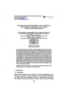
Identification of a Hammerstein system In this example, the support vector regression is used to approximate a Hammerstein system that consists of a series connection of a memory less nonlinearity, f, and linear dynamics, G, as shown in Fig. 5 where v represents the transformed input variable.
Figure 5: Hammerstein system For transparent presentation, the Hammerstein system to be identified consists of a first-order linear part, y(k+1) = 0,9·y(k) + 0,1·v(k), and a static nonlinearity represented by a polynomial, v(k) = u(k)2. The identification data consists of 500 input-output data. A support vector regression model was identified with the efficiency summarized in Table 3. Table 3: SVR results on Hammerstein system identification Method SVM RS Applying OLS Merging
Regress data Model output Support vectors Insensitive region
0
RMSE 0,0533 0,0604 0.0650 0.0792
# Rules 22 15 13 12
Hammerstein data Model output Support vectors Model output after reduction
1
-2
-1,5
0
2
Figure 4: The Regress dataset with model output, support vectors and the insensitive region. The SVR technique obtained Nx = 14. This model has been also reduced by the RS method, by which we tried to reduce the model to NR = 10. After doing the modelling steps described in the classification example we achieved the following results (described in Table 2) Table 2. SVR results on Regress data Method SVM RS OLS Merging
RMSE 0,0840 0,0919 0,2261 0,2415
# Rules 14 10 9 6
The OLS reduction indicated, that reducing with one rule results the increase of modelling error at this example, for an interesting point we mention that using extreme reduction steps in this example (NR = 4, after OLS ranking NR = 2) gives also reasonable results (RMSE = 1.241).
0 250
500
Figure 5: Identified Hammerstein system support vectors and model output after reduction. As Fig. 5 and Table 3 conclude, support vector regression is able to give accurate model for Hammerstein system with, however the results are not interpretable. Hereby the three-step reduction algorithm is used to acquire interpretable fuzzy regression model. After applying the RS method we were able to reduce the number of support vectors to 15 without the loss of the modelling error, but the obtained results are still not interpretable as it can be seen on Fig. 6. Using further reduction with the second and third step of the algorithm OLS and fuzzy membership function merging finally results interpretable (Fig. 7) and accurate (Table 3) fuzzy model.
107 1 0.8 0.6 0.4 0.2 0 0
0.1
0.2
0.3
0.4
0.5
0.6
0.7
0.8
0.9
1
0.1
0.2
0.3
0.4
0.5
0.6
0.7
0.8
0.9
1
1 0.8 0.6 0.4 0.2 0 0
Figure 6: Non-distinguishable membership functions obtained after the application of the RS method 1
ACKNOWLEDGEMENT
0.8 0.6 0.4 0.2 0 0
identification as a regression problem. The obtained models are very compact but their accuracy is still adequate. Besides, it might be clear that still real progress can be made in the development of novel methods for feature selection. We intend this paper also as a case study for further developments in the direction of a combination-of-tools methodology for modelling and identification, aiming at models that perform well on multiple criteria, considering here different soft-computing tools, namely support vector machines and fuzzy techniques are combined to achieve a predefined trade-off between performance and transparency.
0.1
0.2
0.3
0.4
0.5
0.6
0.7
0.8
0.9
1
0.1
0.2
0.3
0.4
0.5
0.6
0.7
0.8
0.9
1
1 0.8 0.6
The authors would like to acknowledge the support of the Cooperative Research Centre (VIKKK) (project 2004-I) and Hungarian Research Found (OTKA T049534). János Abonyi is grateful for the support of the Bolyai Research Fellowship of the Hungarian Academy of Sciences.
0.4 0.2 0 0
Figure 7: Interpretable membership functions of the reduced fuzzy model Conclusion It has been shown in a mathematical way that support vector based techniques and fuzzy rule-based models work in a similar manner as both models maps the input space of the problem into a feature space with the use of either nonlinear kernel or membership functions. The main difference between support vector based and fuzzy rule-based systems is that fuzzy systems have to fulfil two objectives simultaneously, i.e., they must provide a good modelling performance and must also be linguistically interpretable, which is not an issue for support vector systems. However, as the structure identification of fuzzy systems is a challenging task, the application of kernel-based methods for model initialization could be advantageous because of the high performance and the good generalization properties of these type of models. Accordingly, support vector-based initialization of fuzzy rule-based model is used in this paper. First, the initial fuzzy model is derived by means of the support vector learning algorithm. Then the support vector model is transformed into an initial fuzzy model that is subsequently reduced by means of the reduced set method, similarity-based fuzzy set merging, and orthogonal transform-based rule-reduction. Because these rule-base simplification steps do not utilize any nonlinear optimization tools, it is computationally cheap and easy to implement. The application of the proposed approach is shown for the Wisconsin Breast Cancer as a classification problem and Regress data and Hammerstein system
REFERENCES 1. ABONYI J., FEIL B.: Computational Intelligence in Data Mining, Informatica 29 (2005) 3-12 2. KECMAN V.: Learning and Soft Computing, MIT Press 2001 3. ZADEH L. A.: Fuzzy logic, neural networks, and soft computing, Communications of the ACM, Vol. 37 (1994), Issue 3, 77-84 4. SCHÖLKOPF B., MIKA S., BURGES C. J. C., KNIRSCH P., MÜLLER K.-R., RATSCH G., SMOLA A.: Input space vs. feature space in kernel-based methods, IEEE Trans. on Neural Networks, Vol. 10(5) (1999) 5. SETNES M., BABUSKA R., KAYMAK U., VAN NAUTA LEMKE H. R.: Similarity measures in fuzzy rule base simplification, IEEE Trans. SMC-B, Vol. 28 (1998), 376-386 6. YEN J., WANG L.: Simplifying fuzzy rule-based models using orthogonal transformation methods, IEEE Trans. SMC-B Vol. 29, (1999), 13-24 7. SETNES M., HELLENDOORN H.: Orthogonal transforms for ordering and reduction of fuzzy rules, in FUZZIEEE 700-705,San Antonio, Texas, USA 2000 8. CORTES C., VAPNIK V.: Support-Vector Networks, AT&T Research Labs, USA 1995 9. SMOLA A. J., SCHÖLKOPF B.: A tutorial on support vector regression, Statistics and Computing 14, 199-222, 2004 10. TAKAGI T., SUGENO M.: Fuzzy identification of systems and its application to modelling and control, IEEE Trans. SMC Vol. 15 (1985) 116-132 11. GUNN S. R.: Support Vector Machines for Classification and Regression, Technical Report 1998
108 12. SETNES M., BABUSKA R., KAYMAK U., VAN NAUTA LEMKE H. R.: Similarity measures in fuzzy rule base simplification 13. JIN Y.: Fuzzy Modelling of High-Dimensional Systems, IEEE Trans. FS Vol. 8 (2000) 212-221 14. YEN J., WANG L.: Simplifying fuzzy rule-based models using orthogonal transformation methods, IEEE Trans. SMC-B Vol. 29 (1999) 13-24