Interpretation of Compositional Regression with Application to Time

Austrian Journal of Statistics February 2018, Volume 47, 3–19. http://www.ajs.or.at/ AJS

doi:10.17713/ajs.v47i2.652

Interpretation of Compositional Regression with Application to Time Budget Analysis Ivo Mu ¨ ller

Karel Hron

Eva Fiˇ serov´ a

Palack´ y University

Palack´ y University

Palack´ y University

ˇ Jan Smahaj

Panajotis Cakirpaloglu

Jana Vanˇ c´ akov´ a

Palack´ y University

Palack´ y University

Prostor Plus

Abstract Regression with compositional response or covariates, or even regression between parts of a composition, is frequently employed in social sciences. Among other possible applications, it may help to reveal interesting features in time allocation analysis. As individual activities represent relative contributions to the total amount of time, statistical processing of raw data (frequently represented directly as proportions or percentages) using standard methods may lead to biased results. Specific geometrical features of time budget variables are captured by the logratio methodology of compositional data, whose aim is to build (preferably orthonormal) coordinates to be applied with popular statistical methods. The aim of this paper is to present recent tools of regression analysis within the logratio methodology and apply them to reveal potential relationships among psychometric indicators in a real-world data set. In particular, orthogonal logratio coordinates have been introduced to enhance the interpretability of coefficients in regression models.

Keywords: regression analysis, compositional data, time budget structure, orthogonal logratio coordinates, interpretation of regression parameters.

1. Introduction Regression analysis becomes challenging when compositional data as observations carrying relative information (Aitchison 1986; Pawlowsky-Glahn, Egozcue, and Tolosana-Delgado 2015) occur in the role of response or explanatory variables. Although this might frequently seem to be a purely numerical problem, compositional data in any form inducing a constant sum constraint (proportions, percentages) rather represent a conceptual feature. In fact, compositional data may not necessarily be expressed with a constant sum of components (parts). The decision whether data at hand are compositional or not depends on the purpose of analysis - whether it is absolute values of components, or rather their relative structure, that is of primary interest. One of most natural examples of compositional data are time budget (time allocation) data, discussed already in the seminal book on compositional data analysis (Aitchison 1986, p. 365). Apart from the compositional context, due to its psychological, social, and economic

4

Interpretation of Compositional Regression

impacts, time allocation and its statistical analysis receives attention in many publications. The distribution of the total amount of time among productive-, maintenance-, and leisure activities reflects the current status and soundness of economy, with its labour-saving inventions, communication technologies, means of transportation, information and mass media channels, and level of consumption (Becker 1965; Garhammer 2002; Gershuny 2000; Juster and Stafford 1991; Robinson and Godbey 1997). The economy is usually closely linked to political arrangement, which through welfare state institutions (including child-care facilities) relieve citizens of many obligations, thus opening possibilities for loosening and restructuring their daily schedules (Korpi 2000; Gershuny and Sullivan 2003; Crompton and Lyonette 2006). Leisure time service is further provided for by various sports programs, holiday resorts, outdoor activities and the like, for both adolescents and adults. Moreover, frequently also supplementary qualitative/quantitative variables (age, gender, variables resulting from psychometric scales) are of simultaneous interest, which calls for the use of regression modelling. When considering the problem of time allocation from the statistical point of view, the individual activities represent relative contributions to the overall time budget. Particularly, although the input data can be obtained either in the original time units, or directly in proportions or percentages, the relevant information is conveyed by ratios between the parts (time activities). Consequently, also differences between relative contributions of an activity should be considered in ratios instead of absolute differences as they better reflect relative scale of the original observations. Both scale invariance and relative scale issues are completely ignored when the raw time budget data or any representation thereof (like proportions or percentages) are analysed using standard statistical methods. Although there do exist methods whose aim is to solve purely numerical problems resulting from the nature of observations carrying relative information (being of one dimension less than the actual number of their parts), these methods usually do not represent a conceptual solution to the problem of compositional data analysis. Instead, any reasonable statistical methodology for this kind of observations should be based on ratios between parts, or even logratios (logarithm of ratios), which are mathematically much easier to handle (Aitchison 1986; Pawlowsky-Glahn et al. 2015). Logratios as a special case of a more general concept of logcontrasts are used to construct coordinates with respect to the Aitchison geometry that captures all the above mentioned natural properties of compositions. Nevertheless, possibly due to apparent complexity of the logratio methodology, logratio methods haven’t still convincingly entered applications in social sciences, specifically psychological applications; methods to analyse time budget, mentioned in the seminal book of Van den Ark (van den Ark 1999) and resulting from fixing the unit-sum constraint of compositional data, were mostly overcome during the last 15 years of intensive development in the field of compositional data. Very recently statistical analysis of psychological (ipsative) data seems to attract attention (Batista-Foguet, Ferrer-Rosell, Serlav´os, Coenders, and Boyatzis 2015; van Eijnatten, van der Ark, and Holloway 2015). Nevertheless, still rather specific methods are used without providing a concise data analysis, particularly concerning regression modelling that frequently occurs in psychometrics. For this reason, the aim of this paper is to perform a comprehensive regression analysis of time budget structure of college students by taking real-world data from a large psychological survey at Palack´ y University in Olomouc (Czech Republic). With that view, relations with other response/explanatory variables (as well as those within the original composition) will be analysed using proper regression modelling. The structure of the paper is as follows. In the next section, the orthonormal logratio coordinates are introduced first, and then regression modelling is discussed in more detail in Section 3. In order to achieve better interpretability of regression parameters while preserving all important features of regression models for compositional data, orthogonal coordinates (instead of orthonormal ones) are introduced as an alternative in Section 4. Section 5 is devoted to logratio analysis of the concrete time budget data set and the final Section 6 (Discussion) concludes.

Austrian Journal of Statistics

5

2. Orthonormal logratio coordinates for compositional data For a D-part composition x = (x1 , . . . , xD )0 , considering all possible logratios ln(xi /xj ), i, j = 1, . . . , D, for statistical analysis means to take into account D(D − 1)/2 variables (up to sign of the logarithm). This would lead to a complex ill-conditioned problem already for data sets with moderate number of variables. Moreover, information related to the original parts (although expressed possibly in logratios) is usually of primary interest. For this reason, a natural P choice is to aggregate logratios meaningfully to logcontrasts (variables of type D i=1 ci ln xi , PD where i=1 ci = 0), that are able to capture all the relative information about single compositional parts (time activities). In other words, when x1 playsq the role of such a part, we proceed

to variable ln(x1 /x2 ) + . . . + ln(x1 /xD ) = (D − 1) ln(x1 / D−1 D i=2 xi ), i.e. to logcontrast that highlights the role of x1 (?). In order to build a system of orthonormal coordinates, this variable needs to be further scaled and also the remaining D − 2 coordinates, orthonormal log-contrasts, are constructed consequently (we refer to isometric logratio (ilr) coordinates (Egozcue, Pawlowsky-Glahn, Mateu-Figueras, and Barcel´o-Vidal 2003)). One possible choice of ilr coordinates that fulfil the above requirements (for any of parts xl , l = 1, . . . , D, in place (l) (l) of x1 ) is z(l) = (z1 , . . . , zD−1 )0 , Q

s (l)

zi =

D−i ln D−i+1

(l)

x qQ i

D−i

(l) D j=i+1 xj

, i = 1, . . . , D − 1.

(1)

The case of x1 would be obtained by choosing l = 1. In a more general setting, the composition (l) (l) (l) (l) (l) (x1 , x2 , . . . , xl , xl+1 , . . . , xD )0 stands for such a permutation of the parts (x1 , . . . , xD )0 that always the l-th compositional part fills the first position, (xl , x1 , . . . , xl−1 , xl+1 , . . . , xD )0 . In (l) such a configuration, the first ilr coordinate z1 explains all the relative information (merged into the corresponding logcontrast) about the original compositional part xl , the coordinates (l) (l) z2 , . . . , zD−1 then explain the remaining logratios in the composition. Note that the only (l)

(l)

important position is that of x1 (because it can be fully explained by z1 ), the other parts can be chosen arbitrarily, because different ilr coordinates are orthogonal rotations of each other (Egozcue et al. 2003). Although this particular choice of ilr coordinates has been used successfully in many geological and chemometrical applications (Buccianti, Egozcue, and Pawlowsky-Glahn 2014; Filzmoser, Hron, and Reimann 2012; Kalivodov´a, Hron, Filzmoser, Najdekr, Janeˇckov´ a, and Adam 2015), no experiences are recorded in the psychometrical context.

3. Regression analysis within the logratio methodology Regression analysis is an important tool for analysing the relationships between the response variable Y and known explanatory variables x, see, e.g. (Montgomery, Peck, and Vining 2006). Although in the psychometrical context it is often difficult to distinguish whether the covariates are driven by an error as well, or not, we will follow the assumption of fixed covariates in order to enable estimation of regression parameters using the standard least squares (LS) method, resulting in easy-to-handle statistical inference (hypotheses testing). When the response variables or explanatory variables are compositional, special treatment in regression is necessary. A natural way for introducing regression with compositional explanatory variables x = (x1 , x2 , . . . , xD )0 is to perform a standard multiple regression where the explanatory variables zi = (1, zi,1 , zi,2 , . . . , zi,D−1 )0 represent the ilr coordinates of xi and 1 for the intercept (Hron, Jel´ınkov´ a, Filzmoser, Kreuziger, Bedn´aˇr, and Bart´ak 2012). Using a special choice of ilr coordinates z(l) given by (1), we can consider the lth ilr basis, for l = 1, 2, . . . , D, and we obtain D different multiple regression models in the form (l) (l)

(l)

(l)

(l)

Yi = β0 + β1 zi,1 + · · · + βD−1 zi,D−1 + εi , i = 1, 2, . . . , n,

(2)

6

Interpretation of Compositional Regression (l)

(l)

(l)

where β0 , β1 , . . . βD−1 are unknown regression parameters and εi are random errors in the lth model. Due to the orthogonality of different ilr bases, the intercept term β0 is the same for all D models (similarly as the index of determination R2 or the F statistic to test the overall significance of the covariates) (Hron et al. 2012). The regression parameters can be estimated in the standard way by the least squares (LS) method. Using the notation (l) (l) (l) Y = (Y1 , Y2 , . . . , Yn )0 for the observation vector, Z(l) = (z1 , z2 , . . . , zn )0 for n × D design (l) (l) (l) (l) (l) matrix, β (l) = (β0 , β1 , . . . , βD−1 )0 for regression parameters, and ε(l) = (ε1 , ε2 , . . . , εn )0 for the error term, models (2) can be rewritten in the matrix form Y = Z(l) β (l) + ε(l) , l = 1, 2, . . . , D.

(3)

We can consider that random errors in the lth model are not correlated with the same variance 2 . Then the best linear unbiased estimators of regression parameters β (l) by the LS method σ(l) are b (l) = (Z0(l) Z(l) )−1 Z0(l) Y, l = 1, 2, . . . , D. β (4) (l)

From the practical point of view, only the parameter β1 is important, since it corresponds to (l) (l) the first ilr coordinate z1 that explains all the relative information about the part x1 . The (l) (l) other parameters β2 , . . . , βD−1 do not have such straightforward interpretation. So, we can say, e.g., that the absolute change of the conditional mean of Y with respect to coordinate (l) (l) (l) z1 is about β1 , if other coordinates zj , j = 2, 3, . . . , D − 1 (representing subcomposition (x1 , . . . , xl−1 , xl+1 , . . . , xD )0 ), are fixed. 2 in the lth model (3) is The unbiased estimator of σ(l) (l)

(l)

2 b )0 (Y − Z(l) β b )/(n − D), b(l) σ = (Y − Z(l) β

(5)

that can be used to estimate the variance-covariance matrix of the estimator of regression parameters, (l)

2 b )=σ d b(l) v ar(β (Z0(l) Z(l) )−1 .

(6)

Under assumption of normality of random errors we can perform any standard statistical inference, e.g. test the significance of regression parameters, or to construct confidence intervals for them. The significance of the individual regression parameters in the lth model, l = 1, 2, . . . , D, can be tested by the following statistics: T0 =

βb0 q

(l)

(l)

;

Ti

b(l) {(Z0(l) Z(l) )−1 }1,1 σ

=

βbi q

,

(7)

b(l) {(Z0(l) Z(l) )−1 }i+1,i+1 σ

i = 1, 2, . . . , D − 1. Here the symbol {(Z0(l) Z(l) )−1 }i+1,i+1 denotes the (i + 1)th diagonal element of the matrix (Z0(l) Z(l) )−1 . Under the null hypothesis that regression parameters are (l) zeros, the statistics T0 and Ti each follow a Student t-distribution with n − D degrees of freedom. The statistic T0 is the same irrespective of the choice of l = 1, . . . , D in (2), see (Hron et al. 2012) for details. Of course, the response variable can have also another distribution than normal, i.e. the methodology of generalized linear models (Dobson and Barnett 2008) can be directly implemented. Similarly, when the response variables Y = (Y1 , Y2 , . . . , YD )0 are compositional and explanatory variables x = (x1 , x2 , . . . , xk )0 are non-compositional, one can use the regression models where the response variables Z1 , . . . , ZD−1 represent the ilr coordinates of Y (Egozcue, Daunis-i Estadella, Pawlowsky-Glahn, Hron, and Filzmoser 2011). Using the ilr coordinates (l) (1), where only the first ilr coordinate Z1 is of interest, we obtain D different multiple regression models in the form (l)

(l)

(l)

(l)

(l)

Zi,1 = γ0 + xi,1 γ1 + · · · + xi,k γk + εi , i = 1, 2, . . . , n, l = 1, 2, . . . , D.

(8)

Austrian Journal of Statistics

7

In this case, the interpretation of regression parameters is the following. For example, if (l) x2 , . . . , xk are fixed, then for each change of 1 unit in x1 , the conditional mean of Z1 changes (l) γ1 units. Nevertheless, similarly as for the case of regression with compositional explanatory variables, because the orthonormal coordinates (1) have to be interpreted in terms of scaled logratios under natural logarithm, the interpretation of these “units” and thus also values of regression parameters might get rather complex for practical purposes. Under the usual multiple regression model assumptions, (8) can be expressed in the matrix form (l)

Z1 = Xγ (l) + ε(l) , l = 1, 2, . . . , D, (l)

(l)

(l)

(9)

(l)

where Z1 = (Z1,1 , Z2,1 , . . . , Zn,1 )0 is an observation vector, γ = (γ0 , γ1 , . . . , γk )0 is a vector of regression parameters, and X = (1, x1 , x2 , . . . , xk ) is n × (k + 1) design matrix. Here 1 is a vector of n ones. When the random errors in the lth model are not correlated with the 2 , the best linear unbiased estimator of regression parameters γ (l) by the same variance σe,(l) LS method is (l) b (l) = (X0 X)−1 XZ1 , l = 1, 2, . . . , D, γ (10) with the estimated variance-covariance matrix 2 b (l) ) = σ d be,(l) v ar(γ (X0 X)−1 .

(11)

2 The unbiased estimator of σe,(l) in model (9) is (l)

(l)

2 b (l) )0 (Z1 − Xγ b (l) )/(n − k − 1). be,(l) σ = (Z1 − Xγ

(12)

Again, under assumption of normality of random errors we can test the significance of regression parameters, or construct confidence intervals for them. In this case, the significance of the individual regression parameters in the lth model, l = 1, 2, . . . , D, can be tested by the statistic: (l) γbi (l) q Ui = , i = 0, 1, . . . , k. (13) be,(l) {(X0 X)−1 }i+1,i+1 σ (l)

Under the null hypothesis that regression parameters are zeros, the statistics Ui Student t-distribution with n − k − 1 degrees of freedom.

follow a

Finally, within the logratio methodology we can consider also the case of regression among parts of a composition, in particular, between a part x0 and the rest of compositional parts, x1 , . . . , xD , in a (D+1)-part composition. Following (Buccianti et al. 2014; Hr˚ uzov´a, Todorov, Hron, and Filzmoser 2016), a natural choice is to consider the case of regression with compositional explanatory variables, where the response is formed by coordinate, carrying the relative information of x0 (with respect to compositional covariates), i.e., s

z0 =

D x0 ln qQ . D D+1 D x i=1 i

By construction, z0 is orthonormal to the rest of coordinates, assigned to explanatory parts as in (1).

4. Orthogonal coordinates for compositional regression Although the above regression models in orthonormal logratio coordinates are theoretically well justified, both the normalizing constants to reach orthonormality and the natural logarithm itself result in quite a complex interpretation of the regression parameters. A way out is to move to orthogonal coordinates, where nothing from the above properties of regression

8

Interpretation of Compositional Regression (l)

(l)

modelling in coordinates is lost (in particular, values of Ti and Ui statistics, neither the geometrical features of regression with compositional response (Egozcue et al. 2011)), while, at the same time, a substantial simplification in parameter interpretation is gained. Following (1), these considerations lead to orthogonal coordinates (l)

(l)∗ zi

xi

= log2

qQ

(l) D j=i+1 xj

D−i

, i = 1, . . . , D − 1,

(14)

for l = 1, . . . , D, where the normalizing constants are omitted and the original natural logarithm is replaced by the binary one. Let’s see the effect of using the orthogonal coordinates for all regression models introduced above (parameters of their corresponding versions in orthogonal coordinates (14) are always marked with an asterisk). Considering regression with compositional explanatory variables first, from properties of LS estimation and the relation between logarithms of different bases we get s (l)∗

β0∗ = β0 , β1

= ln(2)

D − 1 (l) β1 , D

generally s

D−i (l) β , i = 1, . . . , D − 1, D−i+1 i and similarly for their estimates and the respective standard errors. Analogously, for models resulting from regression with compositional response we get (l)∗

βi

= ln(2)

s (l)∗ γi

= log2 (e)

D (l) γ , i = 0, . . . , k. D−1 i

Finally, in regression within composition both the above effects are combined, i.e., for D regression models (l) (l)

(l)

(l)

(l)

Zi0 = β0 + β1 zi,1 + · · · + βD−1 zi,D−1 + εi , i = 1, 2, . . . , n,

(15)

(l = 1, . . . , D) we obtain s

β0∗

= log2 (e)

D+1 (l)∗ β0 , βi = D

s

(D + 1)(D − i) (l) β , i = 1, . . . , D − 1. D(D − i + 1) i

Indeed, the interpretation of regression coefficients gets simpler now. For regression with compositional regressors and non-compositional response, first note that a unit additive increment in a log-transformed coordinate z is equivalent to a two-fold multiplicative increase in the relative dominance of the original compositional variable x, if the base-2 logarithm is used, that is, (l) (l) x1 x1 (l)∗ ∆z1 = log2 qQ · 2 − log2 qQ = 1. D−1 D−1 (l) (l) D D x x i=2 i i=2 i (l)∗

The coefficient β1 in the regression equation then has the usual meaning of an additive increase in the response y that corresponds to increasing z by one (i.e., increasing the dominance (l)∗ of x twice), while keeping all else fixed. For example, if β1 = 3, the value of the response gets higher by 3 units when the relative dominance of the part xl with respect to the average of the other parts, see the logratio in (14), is doubled, at constant values of the other involved covariates (orthogonal coordinates). Next, in case of regression with compositional response (l)∗ and non-compositional regressors, γj is the additive increment of the log-transformed response z when adding one to an explanatory variable xj , j = 1, . . . , k, (at constant values of the other covariates) (l)

(l)∗ γj

=

(l)∗ ∆Z1

= log2

Y1 q

D−1

QD

(l)

(l) δ (l) j

i=2 Yi

− log2

Y1 q

D−1

(l) i=2 Yi

QD

(l)

= log2 δj ,

Austrian Journal of Statistics (l)

where δj

9

(l)∗

= 2γj

is the multiplicative increase in the relative dominance of the original (l)

compositional response y. So, for a unit additive change in xj , the ratio of Y1 (l) δj

to the

(l)∗ γj

“mean value” of the other compositional responses grows = 2 times. Finally, an analogous interpretation for regression within composition can be obtained, namely, a twofold multiplicative increase in the relative dominance of xl (or equivalently, a unit additive (l)∗ increment in coordinate z1 ) brings the increase in the relative dominance of the response x0 of (l)

(l)∗

(l)

δ1 = 2β1 , where ∆Z0∗ = log2 δ1 . Note also that the above expression for the proportionality coefficient δ stays the same irrespective of the base to which the logarithm was taken, as factor 2 in the expression now stands for two-fold increase in dominance, not for the logarithmic base.

5. Time budget analysis Following the previous developments, the decision to admit that the time budget data are by their nature compositional invites one to couch analysis in terms of logratios instead of working with the original observations in percentages; namely, the latter would lead to biased conclusions due to relative character of compositions. The aim of this section is to demonstrate on real-world psychometric data that working with logratios in the regression context is as accessible as dealing with the original observations.

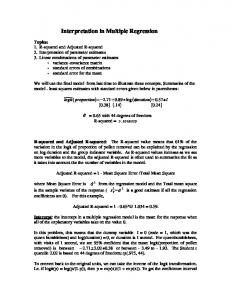
5.1. Data and methods For this purpose, we employ data from (Vanˇc´akov´a 2013) that were obtained in a large psychometric study, guaranteed and realized by the Department of Psychology, Palack´ y University in Olomouc, Czech Republic. A questionnaire called “Leisure Time” was distributed among students at the above university, reaching a total of N = 414 respondents (347 women, 67 men) who provided complete answers. The items included in the questionnaire tapped three distinct areas: i) personal characteristics (age, gender, faculty and field of study); ii) leisure time (its concept, absolute and relative amount, content); iii) personality traits (self-esteem and attitude to challenges). In terms of current analysis, of particular interest are relationships among the following variables: Daily Time Budget as expressed in seven compositional variables (parts, summing up to 100 percent) study/work, commuting, food, hygiene&dressing, sleep, household duties, and leisure time; personality variables self-esteem (z-score from a 10-item Rosenberg Self-Esteem Scale (Rosenberg 1965) included in the questionnaire) and challenge (“Are you a person who invites challenges, i.e. opportunities to surpass yourself?”, originally 4-choice response collapsed into dichotomic and coded as 1 for “always” or “almost always”, and 0 for “almost never” or “never”); and covariates of age (in years) and gender (dichotomic, coded as 1 for men and -1 for women). Distribution of the variables age and self-esteem is visualized in Figure 1 in the form of EDA-plots using the R package StatDA (Filzmoser 2013). Although the respondents were asked to enter data on Daily Time Budget in percentages, the obtained range of the sum of parts was h7, 520i due to misunderstanding the units to use and their prescribed constant sum constraint (of course, most of the row sums were exactly or close to 100). Nevertheless, the important information on relative contributions of parts to the overall time budget was unaffected by using whatever units, which thus emphasizes even further the necessity to apply the logratio methodology in statistical processing. Note once again that for the logratio methodology the constant sum representation of compositional data is not a necessary requirement. However, for the purpose of easier comparisons, in the following the percentage representation was taken for all time budget observations. Besides paying attention to differences, as well as agreement, in logratio vs. “standard”

Interpretation of Compositional Regression

● ●

20

25

60 40 −20

0

20

Frequency

50 0

Frequency

100

80

150

10

●

30

age

35

40

45

● ● ● ●

−3

● ●

−2

−1

0

1

2

3

z−score

Figure 1: EDA-plots for variables age (left) and self-esteem (right).

methodologies, we will keep our thoughts focused on some tentative conjectures about interconnections among variables. This data set allows for exploring possible influences among several prominent psychological factors. On the one hand, we have the pair of personality traits of self-esteem and openness to challenge which we expect to be bundled close together and even boost each other if challenges are being tackled successfully, or else restrain each other in a downward spiral. On the other hand, the necessity of time allocation brings about an inevitable interplay of work, active relaxation, and sleep (passive relaxation). And then, of course, these two broad areas come into mutual contact in complex ways. These considerations lead us, at the outset, to postulate a firm and positive relationship between personality traits of challenge and self-esteem. Next, within compositional variables, we deem as highly probable a negative relationship between work/study and leisure time, and between work/study and sleep on the premise that working/studying takes away time from both these forms of relaxation. Sleep is considered loosely associated with leisure time on the grounds that the time left after deducting all duties is being distributed between both. If there is more time available, it will add up to both sleep and leisure. If any at all, the relationship between sleep and challenge is expected to be negative, as the person who is busy taking challenges might have less time for sleep. The association between sleep and self-esteem is less clear-cut but it can be conceived along the lines that a self-assured person participates in numerous activities and thus sleeps less, while, on the other hand, an insecure person may seek sleep as a welcome escape from reality. As a consequence, work/study should be positively related with both challenge and self-esteem, and leisure time negatively related with both. Any effects of gender may be obscured in this dataset as men are seriously underrepresented among respondents. In the following, the relationships among variables are determined through regression analysis. A logratio approach (which is deemed appropriate whenever a compositional variable out of Daily Time Budget is present) is compared to a standard non-compositional approach, e.g. Linear Model (LM) or Generalized Linear Model (GLM). In the statistical analysis we focused on those relations that are primarily not gender related. Moreover, preliminary exploratory analysis using variation matrix (Aitchison 1986) and compositional biplot (Aitchison and Greenacre 2002), see Figure 2, revealed strong relationship between food and hygiene&dressing components; because of their rather marginal importance for psychological interpretation, these parts will be excluded from further consideration (but kept as parts of the initial composition). On the other hand, there seems to be no relation between commuting

Austrian Journal of Statistics

−0.6

−0.4

−0.2

0.0

0.2

0.4

11

0.6

0.6 −0.4

2

6 −2

−1

0

1

−0.2

0.0

0.2

0.4

. .1 . . . . . . . . . . .. . . . . 5. . . . .. . . . . . . . . .. . . . . . . . . . . . . .. .. .. ... ... .. . . . . .. . . . .. . .. ... ....................... ....... . . . . . . . 7 . . ... .... . . ... .... ..... ... ... . .... . . . . . . . ... . . .. .. . . . .. . . .. ..... . . .. .. . .... . . ... ..... .. .. .... . . . . ... . .... ... . .. ... . .. .. . . . .... . .. ... . .. . .... ...... ............ .... .. ......... . . ... . .. . .. . .... 3. .... ... ... . . . . . . . . . . . . .. .. ........ .. ... . . . .4 . . .. .. ... . ... .. .. . . . .. .. .. .. . . . . . . .. . . . .. . . . . . ..

−0.6

0

.

−2

−1

PC 2 (23.42%)

1

2

.

2

PC 1 (27.02%)

Figure 2: Compositional biplot for time budget data. Number codes correspond to single activities (1 − study/work, 2 − commuting, 3 − food, 4 − hygiene&dressing, 5 − sleep, 6 − household duties, 7 − leisure time) and leisure time, or study/work and household duties, respectively. Interestingly, there is some nearly constant ratio also between study/work and sleep throughout the sampled population, which goes against the hypothesized association.

5.2. Regression analysis From the essence of the data set, interconnections among variables (compositional and noncompositional, or even within the time budget composition) are of primary interest. For this purpose, several regression models were applied to data. Accordingly, in addition to Daily Time Budget, non-compositional variables of challenge, self-esteem, age, and gender were taken into consideration here. In order to enable direct interpretation of regression output, orthogonal coordinates (as described in Section 4), instead of orthonormal ones, were employed for the compositional variables within logratio approach. As a first step, let us explore the manner how seeking challenges is determined by Daily Time Budget and other explanatory variables. That is, the response now is non-compositional (binomial), while some of the regressors are compositional and others not. For this purpose, binomial regression (a special case of logistic regression) was applied, first with compositional regressors in logratio coordinates, second with the original variables in percentages; note that any representation of the orthogonal logratio coordinates would lead to the same parameter estimates for the non-compositional covariates. From the time budget variables just those of potential psychological influence were included (study/work, commuting, sleep, household duties, and leisure time); of course, due to construction of the regression model in coordinates, all parts of the original composition were taken into account for the estimation purposes under logratio approach. On the other hand, perfect collinearity among compositional variables

12

Interpretation of Compositional Regression

makes it impossible to include all of them simultaneously as regressors in a standard linear model. Following (Hron et al. 2012), common regression output like parameter estimates, their standard errors, values of corresponding statistics and their P-values (using function glm from R-package MASS, see (Venables and Ripley 2002) for further details) are collected in Table 1 (all tables with detailed results are included as supplementary material), where names of the original parts stand as notation for the corresponding orthogonal coordinates (14). It can be seen that both the study/work coordinate and the self-esteem variable are contributing the most (in the positive direction, due to positive sign of their coefficients) in explaining the challenge response. The interpretation of coefficients is such that if the relative dominance of study/work in time budget doubles (with respect to average contribution of the other parts), the odds for seeking challenges increases exp(0.422) = 1.53-fold (other covariates staying fixed); similarly, a unit increase in self-esteem z-score brings increase of the odds for seeking challenges exp(0.452) = 1.57-fold. Note that, in line with the methodology described in the previous section, five regression models were employed to obtain the estimates for the compositional coordinates. By applying orthogonal coordinates (14), the interpretation of regression coefficients gets much easier than with original orthonormal coordinates (1). The tight link between challenge and self-esteem is thus established. On the other hand, we don’t see significance of either sleep or leisure time, though the direction (sign of coefficient) is as expected. For all binomial regression models the usual model diagnostics can be done, being the same irrespective which ilr coordinate system for representation of compositional predictors is taken. Specifically, jackknife deviance residuals against linear predictor, normal scores plots of standardized deviance residuals, plot of approximate Cook statistics against leverage/(1-leverage), and case plot of Cook statistic as listed, e.g. in function glm.diag.plots from the package boot can be obtained. In our case normality of residuals is rather limited, though plots of the Cook statistics do not show a significant amount of influential/leverage points that supports reliability of the results. Finally, note that it would be also possible to add interactions between single compositional parts (represented by the respective ilr variables) and non-compositional predictors. An example of that would be possible interaction between variable study/work changing with age, i.e. fresh students and students shortly before finishing the study might have different values on study/work than others. Nevertheless, in order to keep simplified level of the modelling, interactions were not allowed; moreover, even when such a promising interaction was added to the model, the resulting parameter was not significant.

Table 1: Logratio approach: Results from regression of challenge on orthogonal coordinates of the explanatory composition and further covariates. For explanations see text.

(Intercept) study/work commuting sleep household duties leisure time self-esteem age gender

Estimate Std. Error -0.69708 1.24154 0.42200 0.14164 -0.06723 0.10961 -0.20460 0.17476 -0.02904 0.11187 -0.13142 0.12714 0.45187 0.11105 0.04298 0.05516 0.19698 0.15494

Null deviance: 552.4 Residual deviance: 521.4 AIC: 541.4

on 413 on 404

z value Pr(>|z|) -0.561 0.57448 2.979 0.00289 -0.613 0.53959 -1.171 0.24168 -0.260 0.79519 -1.034 0.30129 4.069 4.72e-05 0.779 0.43586 1.271 0.20360

degrees of freedom degrees of freedom

Number of Fisher Scoring iterations: 4

Austrian Journal of Statistics

13

The output of binomial regression with the original compositional variables is shown in Table 2. The interpretation of regression parameters is analogous to standard multiple regression. The exponential function exp(·) of the estimate of regression parameter corresponding to given covariate (either in percentages or in other units) represents amount by which the odds of challenge would increase/decrease if that covariate were one unit higher by constant values of the other covariates. By taking this interpretation into account, there is not much difference from the logratio approach above (also the model fit, expressed by AIC criterion, stays almost the same), which would indicate that the distortion of covariance structure among percentage covariates (see, e.g., (Aitchison 1986) for details) didn’t have dramatic influence on regression output. The strength of association between openness to challenge and selfesteem remains unchanged. Nevertheless, the interesting influence of study/work coordinate, which was clearly visible using the logratio coordinates, is now lost. Table 2: GLM approach: Results from binomial regression of challenge on original explanatory composition (in percentages) and further covariates. For explanations see text.

(Intercept) study/work commuting sleep household duties leisure time self-esteem age gender

Estimate Std. Error z value Pr(>|z|) -0.44332 1.90962 -0.232 0.816 0.02123 0.01853 1.146 0.252 -0.00242 0.03916 -0.062 0.951 -0.00467 0.02077 -0.225 0.822 0.00073 0.03098 0.024 0.981 -0.01892 0.02253 -0.840 0.401 0.44518 0.11046 4.030 5.57e-05 0.03610 0.05418 0.666 0.505 0.16862 0.15198 1.110 0.267

Null deviance: 552.40 Residual deviance: 524.04 AIC: 542.04

on 413 on 405

degrees of freedom degrees of freedom

Number of Fisher Scoring iterations: 4

As a second step, let us look the other way around and search for possible significant covariates of Daily Time Budget. For this purpose regression with compositional response was employed, the response variables now being the five chosen Daily Time Budget variables. The logratio approach leads to five univariate regression models (with orthogonal coordinates corresponding to individual compositional parts) and the results are displayed in Table 3 (to save space, just regression estimates and possible significance at the usual level α = 0.05, marked by asterisk, are provided). The effects of particular covariates on response coordinates are evident. For example, by increasing the value of self-esteem by one, the relative dominance of leisure time in the composition (with respect to average of parts) increases approximately by 6 percent (20.088 = 1.06). Similarly, taking challenges brings the relative dominance of study/work 18 percent higher (20.237 = 1.18), and one more year of age 2.9 percent higher. The positive association between study/work and taking challenges is in accordance with our anticipations, but with self-esteem and leisure time a contrary direction was expected. The connection between sleep and both challenge and self-esteem remained below significance. It is interesting to see also some gender influence on both sleep and leisure time. Due to coding used (1 for male and −1 for female) it can be concluded that for males sleep and leisure time play a more important role in the overall time budget than for females. More (sleep)∗ precisely, the part sleep is explained only by gender. Hence, zb1 = 1.644 is the fitted (sleep)∗ (sleep)∗ value of the coordinate z1 for males, while zb1 = 1.357 for females. It means that the relative dominance of sleep in the composition to the “mean value” of the other compositional responses is 21.644 = 3.125 for males (3.125 times higher relative contribution of sleep than for the averaged rest of components), and 21.357 = 2.562 for females. Further, it can

14

Interpretation of Compositional Regression 2b γ∗

be concluded that the relative dominance of sleep for males is 2 (sleep) = 1.22 times greater than for females. Although results for food and hygiene&dressing variables are in general not discussed in this section, it is worth to note that for hygiene&dressing a significant role of gender (in the negative sense) was revealed; accordingly, this compositional part plays a more important role in time budget of females than for males. Table 3: Logratio approach: Results from regression with compositional response. Significant regression parameters (at α = 0.05) marked by asterisk. study/work (Intercept) 0.60673 challenge 0.23723* self-esteem -0.02201 age 0.04117* gender -0.03217

commuting -1.17704 -0.02216 0.02367 -0.00789 -0.05116

sleep 1.50068* -0.01922 0.03083 0.00186 0.14381*

household -1.27186* -0.07174 -0.01959 0.02723 -0.04412

leisure time 0.96194* -0.13237 0.08817* -0.01801 0.22449*

By way of comparison, the same regression model was analysed under the assumption of Dirichlet distribution for the compositional response that is popular also in psychometric context (Georguieva, Rosenheck, and Zelterman 2008) and, although rather inconsistent with logratio methodology, is still frequently recommended for modelling compositional data. For this purpose function DirichReg from the package DirichletReg (Maier 2014) was applied by expressing the input compositions in proportional representation; regression output is collected in Table 4. The interpretation of regression parameters is analogous to standard multiple regression by considering proportional representation of the response and the fact that parameters of the Dirichlet distribution, being not scale invariant, are predicted. Apart from apparent computational complexity of the model, Dirichlet regression does not seem to shed new light into the problem; moreover, some of the potential relationships that have emerged with the logratio approach are lost again. Table 4: GLM approach: Results from Dirichlet regression with compositional response. Significant regression parameters (at α = 0.05) marked by asterisk. study/work (Intercept) 2.05549* challenge 0.08550 self-esteem 0.03210 age 0.00825 gender -0.03630

commuting 0.94065* -0.05467 0.04770 -0.01401 -0.03837

sleep 2.59815* -0.06799 0.06618 -0.01578 0.06755

household 0.98208 -0.08346 0.02641 -0.00027 -0.03792

leisure time 2.21778* -0.14143 0.09649* -0.02443 0.11748*

From the previous analysis, leisure time seems to be strongly linked with the non-compositional variables. A natural question thus arises whether regression could reveal also some relations within parts of the time budget composition. Thus, as the third step, the corresponding logratio model from Section 2 was applied, by expressing both the response and regressors in orthogonal logratio coordinates (and with additional non-compositional covariates). Similarly as before, Table 5 collects results from four regression models, each highlighting the role of one of compositional explanatory variables (without influence on the non-compositional covariates). Though the R2 statistic gives rather low value (as is usual in social science), some patterns stand out. In particular, relative dominance of leisure time is positively influenced by sleep (increasing the dominance of sleep twice enlarges the dominance of leisure time by 27 percent, as 20.34 = 1.27) and marginally by self-esteem (unit increase in self-esteem increases the dominance of leisure time by 6 percent); negative effects on leisure time are formed by study/work (10 percent decrease in dominance, 2−0.16 = 0.90) and commuting (decrease in

Austrian Journal of Statistics

15

dominance by 13 percent). Consistency with the previous logratio model (Table 3, regression with compositional response) is underlined by the roles of self-esteem and gender covariates. Again, a psychological interpretation can be easily derived. Here we are able to pinpoint the significant positive association of sleep and leisure time, as well as negative association of work/study and leisure time. Marginally significant is the connection between leisure time and self-esteem which appeared significant in previous regression (Table 3). Table 5: Logratio approach: Results from regression of leisure time coordinate on orthogonal coordinates of the explanatory composition and further covariates. For explanations see text.

(Intercept) study/work commuting sleep household duties challenge self-esteem age gender

Estimate Std. Error 0.47988 0.45492 -0.15646 0.05576 -0.20414 0.04377 0.33976 0.06374 0.05734 0.04304 -0.09358 0.08937 0.08353 0.04330 -0.01908 0.01991 0.16760 0.05951

t value Pr(>|t|) 1.055 0.29211 -2.806 0.00526 -4.664 4.22e-06 5.330 1.64e-07 1.332 0.18351 -1.047 0.29568 1.929 0.05442 -0.958 0.33852 2.817 0.00509

Residual standard error: 0.8544 on 404 degrees of freedom Multiple R-squared: 0.1619, Adjusted R-squared: 0.1433 F-statistic: 8.674 on 9 and 404 DF, p-value: 6.21e-12

For the final comparison we consider the standard linear regression model where the original parts in percentages are involved (except for food and hygiene&dressing), see Table 6 for the regression summary. Although conclusions from this model as regards non-compositional covariates would be pretty similar as with logratio methodology, the situation is different in other respects. By comparing R2 for these two models and P-values at respective compositional covariates it is easy to see that for the standard regression model these values are very strongly driven by the constant-sum constraint of the original composition. In particular, note that by including all the compositional parts, R2 would be brought up to 1, i.e., relations between the response and covariates would be completely driven by constant sum constraint of the input data. Of course, as statistical processing of the original compositions violates both scale invariance and relative scale properties of observations, it cannot be concluded that by considering compositional data without a constant sum constraint, the resulting regression model would be relevant. Nevertheless, in percentage representation, which is the case here, the irrelevance of the standard approach is clearly observable.

5.3. Results The logratio approach to regression analysis supports our hypothesis of strong negative association between work/study and leisure time, as well as of strong positive association between challenge and self-esteem. Next, leisure time is significantly tied to self-esteem but the direction here appeared positive, rather than negative as expected. The reason could be that self-assured people don’t feel the urge to work that much and rather take things easy, allowing ˇıpek 2001) says that people themselves more leisure. Also, an explanation in keeping with (S´ with higher self-esteem may be better prepared to use their free time and it may be easier for them to admit their needs (for rest and reward). The connection between leisure time and challenge was not born out (remained below significance, though direction was negative as anticipated). The above regression results were agreed on by both logratio and standard linear model approaches. Both approaches also showed a relationship between sleep and leisure time. However, here the directions differed: logratio showed it to be positive (as hypothesized), linear model negative. On top of that, logratio approach was capable of revealing a

16

Interpretation of Compositional Regression

Table 6: Standard LM approach: Results from regression of leisure time on other compositional parts (in percentages) and further covariates. For explanations see text. Coefficients: (Intercept) work/study commuting sleep household duties challenge self-esteem age gender

Estimate Std. Error 56.88605 2.96589 -0.60560 0.02698 -0.94166 0.07235 -0.51838 0.03738 -0.63007 0.06094 -0.41193 0.48376 0.46017 0.23468 0.05062 0.10826 1.00488 0.31835

t value Pr(>|t|) 19.180 < 2e-16 -22.446 < 2e-16 -13.016 < 2e-16 -13.869 < 2e-16 -10.339 < 2e-16 -0.852 0.39498 1.961 0.05058 0.468 0.64032 3.157 0.00172

Residual standard error: 4.636 on 405 degrees of freedom Multiple R-squared: 0.6014, Adjusted R-squared: 0.5935 F-statistic: 76.37 on 8 and 405 DF, p-value: < 2.2e-16

significant positive connection between challenge and work/study. The psychologically relevant variables seem to form a well-defined cluster of challenge, selfesteem, and work/study. Somewhat in opposition stands the pair of leisure time and sleep. However, their position with respect to the main cluster is less clearly marked, as leisure time is negatively linked to work/study but positively (perhaps only marginally) to self-esteem. Nevertheless it seems reasonable to assume that working/studying does take time away from both leisure and sleep simultaneously. Finally, it is also worth noting that standard regression models were presented mostly for the sake of comparison of the logratio approach with alternatives that would be most possibly used instead. While in some cases their output might seem meaningful, it can also happen that by ignoring the relative structure of Daily Time Budget some interesting features are lost, as was the case in Table 2 and Table 4. For some cases, like when percentage representation of the relative contributions is analysed, it is very easy to demonstrate that scale invariance of compositional data leads to clear failure of the standard approach (Table 6).

6. Discussion Specific habits of time allocation reveal a lot about an individual, a community, a society, or a culture. In each society, options available to individuals for earning their living determine the amount of time they will spend working, or preparing themselves for any such productive activity through study or apprenticeship. In modern times, we have witnessed a continuous reduction in working hours, at least in industrialized countries. At the same time, due to constant total time budget, this development leaves more space for other activities, both necessary (self- and home-maintenance like sleep, eating, hygiene, care for family and house) and discretionary (leisure activities like socializing, culture, sports, reading, idling, etc.). As the time budget data are usually accompanied with other psychometric variables, regression modelling is the first and intuitive choice for a relevant statistical analysis. Due to relative character of time budget allocation, it seems natural to work with (log-)ratios rather than with observations in the original scale (i.e. represented usually in proportions or percentages). It turned out that logratios meet the scale invariance and relative scale requirements (among others that are important for reasonable processing of compositional data) commonly raised in connection with any observations carrying primarily relative information. The main problem is then how to construct logratio coordinates, both meaningful from the mathematical point of view (guaranteed in particular by orthonormality of coor-

Austrian Journal of Statistics

17

dinates) and at the same time providing easy interpretation. The aim of the paper was to enhance interpretability of regression analysis output by employing orthogonal coordinates in place of the mathematically preferred orthonormal ones, demonstrated for the particular case of time budget data. The reason for the choice of alternative coordinates is that all the beneficial properties of the orthonormal coordinates are maintained also by the orthogonal ones, but the latter enable (by avoiding the scaling constants and changing the logarithmic base) a more straightforward interpretation. We are convinced that better interpretability of the regression models, discussed in the paper, can help with applicability of the logratio methodology in psychological research, and also in general.

Acknowledgements The authors gratefully acknowledge the support of the Operational Program Education for Competitiveness - European Social Fund (project CZ.1.07/2.3.00/20.0170 of the Ministry of Education, Youth and Sports of the Czech Republic) and the grant COST Action CRoNoS IC1408.

References Aitchison J (1986). The Statistical Analysis of Compositional Data. Chapman and Hall, London. Aitchison J, Greenacre M (2002). “Biplots of Compositional Data.” Journal of the Royal Statistical Society: Series C (Applied Statistics), 51, 375–392. Batista-Foguet JM, Ferrer-Rosell B, Serlav´os R, Coenders G, Boyatzis RE (2015). “An Alternative Approach to Analyze Ipsative Data. Revisiting Experiential Learning Theory.” Frontiers in Psychology, 6(1742). Becker GS (1965). “A Theory of the Allocation of Time.” The Economic Journal, 75(299), 493–517. Buccianti A, Egozcue JJ, Pawlowsky-Glahn V (2014). “Variation Diagrams to Statistically Model the Behavior of Geochemical Variables: Theory and Applications.” Journal of Hydrology, 519, 988–998. Crompton R, Lyonette C (2006). “Work-life ‘Balance’ in Europe.” Acta Sociologica, 49(4), 379–393. Dobson AJ, Barnett AG (2008). An Introduction to Generalized Linear Models. CRC Press, Boca Raton. Egozcue JJ, Daunis-i Estadella J, Pawlowsky-Glahn V, Hron K, Filzmoser P (2011). “Simplicial Regression: The Normal Model.” Journal of Applied Probability and Statistics, 6(1&2), 87–108. Egozcue JJ, Pawlowsky-Glahn V, Mateu-Figueras G, Barcel´o-Vidal C (2003). “Isometric Logratio Transformations for Compositional Data Analysis.” Mathematical Geology, 35(3), 279–300. Filzmoser P (2013). “StatDA: Statistical Analysis for Environmental Data. R package version 1.6.7.” URL http://CRAN.R-project.org/package=StatDA. Filzmoser P, Hron K, Reimann C (2012). “Interpretation of Multivariate Outliers for Compositional Data.” Computers & Geosciences, 39, 77–85.

18

Interpretation of Compositional Regression

Garhammer M (2002). “Pace of Life and Enjoyment of Life.” Journal of Happiness Studies, 3, 217–256. Georguieva R, Rosenheck R, Zelterman D (2008). “Dirichlet Component Regression and Its Applications to Psychiatric Data.” Computation Statistics & Data Analysis, 52, 5344–5355. Gershuny J (2000). Changing Times. Work and Leisure in Postindustrial Society. Oxford University Press, Oxford. Gershuny J, Sullivan O (2003). “Time Use, Gender and Public Policy Regimes.” Social Politics, 10, 205–228. Hron K, Jel´ınkov´ a M, Filzmoser P, Kreuziger R, Bedn´aˇr P, Bart´ak P (2012). “Statistical Analysis of Wines Using a Robust Compositional Biplot.” Talanta, 90, 46–50. Hr˚ uzov´a K, Todorov V, Hron K, Filzmoser P (2016). “Classical and Robust Orthogonal Regression between Parts of Compositional Data.” Statistics, 50(6), 1261–1275. Juster FT, Stafford FP (1991). “The Allocation of Time: Empirical Findings, Behavioral Models, and Problems of Measurement.” Journal of Economic Literature, 29(2), 471–522. Kalivodov´ a A, Hron K, Filzmoser P, Najdekr L, Janeˇckov´a H, Adam T (2015). “PLS-DA for Compositional Data with Application to Metabolomics.” Journal of Chemometrics, 29, 21–28. Korpi W (2000). “Faces of Inequality: Gender, Class and Patterns of Inequalities in Different Types of Welfare States.” Social Politics, 7, 127–191. Maier MJ (2014). “DirichletReg: Dirichlet Regression in R. R package version 0.5-2.” URL http://dirichletreg.r-forge.r-project.org/. Montgomery DC, Peck EA, Vining GG (2006). Introduction to Linear Regression Analysis. John Wiley & Sons, Hoboken. Pawlowsky-Glahn V, Egozcue JJ, Tolosana-Delgado R (2015). Modeling and Analysis of Compositional Data. Wiley, Chichester. Robinson JP, Godbey G (1997). Time for Life: The Surprising Way Americans Use Their Time. Pennsylvania University Press, University Park (PA). Rosenberg M (1965). Society and the Adolescent Self-image. Princeton University Press, Princeton. van den Ark LA (1999). Contributions to Latent Budget Analysis: A Tool for the Analysis of Compositional Data. DSWO-press, Leiden. van Eijnatten FM, van der Ark LA, Holloway SS (2015). “Ipsative Measurement and the Analysis of Organizational Values: an Alternative Approach for Data Analysis.” Quality & Quantity, 49, 559–579. Vanˇc´akov´a J (2013). “Game, Free Time and the Individual (in Czech).” URL http://www. vmonline.cz/cz/hra-volny-cas-a-jedinec-vancakova-2013/. Venables WN, Ripley BD (2002). Modern Applied Statistics with S. Springer, New York. ˇıpek J (2001). Introduction to Geopsychology: The World and Wanderings Through It in a S´ Context of Recent Times (in Czech). ISV Publishing House, Praha.

Austrian Journal of Statistics

19

Affiliation: Ivo M¨ uller, Karel Hron, Eva Fiˇserov´ a Department of Mathematical Analysis and Applications of Mathematics Faculty of Science Palack´ y University 17. listopadu 12 CZ-77146 Olomouc, Czech Republic E-mail: [email protected], [email protected], [email protected] ˇ Jan Smahaj, Panajotis Cakirpaloglu Department of Psychology Philosophical Faculty Palack´ y University Vod´arn´ı 6 771 80 Olomouc, Czech Republic E-mail: [email protected], [email protected] Jana Vanˇc´ akov´ a Prostor Plus Na Pustinˇe 1068, 280 02 Kol´ın, Czech Republic E-mail: [email protected]

Austrian Journal of Statistics published by the Austrian Society of Statistics Volume 47 February 2018

http://www.ajs.or.at/ http://www.osg.or.at/ Submitted: 2017-02-23 Accepted: 2017-11-28