Basic issues on the use of t-norms for approximate reasoning with interval fuzzy sets are addressed. Inference rules are given for using both numeric intervals ...
Interval based Uncertain Reasoning using Fuzzy and Rough Sets Y.Y. Yao Jian Wang Department of Computer Science Lakehead University Thunder Bay, Ontario Canada P7B 5E1
Abstract This paper examines two interval based uncertain reasoning methods, one is based on interval fuzzy sets, and the other is based on rough sets. The notion of interval triangular norms is introduced. Basic issues on the use of t-norms for approximate reasoning with interval fuzzy sets are addressed. Inference rules are given for using both numeric intervals and lattice based intervals. The theory of rough sets is used to approximate truth values of propositions and to explore modal structures in many-valued logic. Reasoning based on rough sets is complementary to reasoning based on interval fuzzy sets.
1.
Introduction
A fuzzy set is defined in terms of a function from a universe to the unit interval [0, 1]. That is, the membership of each element belonging to a fuzzy set is a single value between 0 and 1. The intersection and union of fuzzy sets are defined in terms of min-max system, probabilistic-like system, and more generally triangular norms and conorms (t-norms and t-conorms for short). Such a single-value-based system is commonly known as the type-1 fuzzy set system. In practical applications, there is also a need to represent the membership of an element by using a fuzzy set in [0, 1], instead of a single value. This system is known as the type-2 fuzzy set system. Operations on type-2 fuzzy sets are defined by extending the operations on the fuzzy sets representing element memberships. Studies on operations of type-2 fuzzy sets have been concentrated mainly on the min-max system [6, 19]. In addition, inference with type-2 fuzzy sets is computationally expensive. In order to overcome this difficulty, special cases of type-2 fuzzy sets have been considered [9, 23]. For example, fuzzy sets representing memberships 1
of elements may be restricted to fuzzy intervals of [0, 1]. If ordinary subintervals of [0, 1] are used to represent membership, one obtains the interval fuzzy sets commonly known as Φ-fuzzy sets [23]. Although it is important to study type-2 fuzzy sets, in the general case, based on the calculus of fuzzy quantities [9], it is equally important to study some special cases. The particular characteristics of each special case may offer more efficient algorithms and more insights that may not be obtained in the general case. For example, one can derive closed-form solutions of fuzzy set operations for fuzzy intervals [9]. Kenevan and Neapolitan [13] studied interval fuzzy sets based on the usual min-max system. Dubois and Prade [9], and Goodman et al. [12] studied the same problem of extending min-max system to interval fuzzy sets, in connection to Lukasiwicz manyvalued logic and interval analysis. Turksen [25] discussed the notion of interval-valued fuzzy sets constructed from the disjunctive and conjunctive normal forms, DNF and CNF, in which certain types of t-norms can be used. Operations on interval-valued fuzzy sets are defined by considering all possible combinations of DNF and CNF [26]. On the other hand, in Φfuzzy sets, an interval is merely regarded as the range within which lies the true membership [13, 23]. The computation of fuzzy set operations may be simplified. Dubois and Prade [8] introduced the notion of twofold fuzzy sets, which is a special kind of Φ-fuzzy sets such that the lower bound of a twofold fuzzy set is included in the core of the upper bound. More specifically, the lower and upper bounds are interpreted as bounds of necessity and possibility. Consequently, the min-max system is used to define operations on twofold fuzzy sets. Bonissone [1, 2] proposed an approximate reasoning model with interval representation of uncertainty, in which four operations are defined using t-norms. The theory of rough sets offers a different interval based method. The interval approximations stem from a lack of sufficient information or incomplete information. A set is assumed to be precisely defined. However, the available information, given in terms of equivalent classes, does not allow us to describe the set exactly. In other words, it may be impossible to describe a precisely defined set with equivalence classes. In this case, a pair of lower and upper approximations is obtained. The lower approximation contains all elements necessarily belonging to the set, while the upper approximation contains all elements possibly belonging to the set. Inference with rough sets can be done in a similar manner, as in modal logic [30]. The results of the above studies motivate the present investigation of interval based uncertain reasoning using fuzzy and rough sets. One of the main objectives of this paper is to study extended t-norms (called interval t-norms) for interval fuzzy set operations. Interval t-norms are defined as two-place functions on the closed subintervals of [0, 1] by drawing results 2
from interval computation. Using interval t-norms, operations on interval fuzzy sets can be efficiently computed, i.e., by computing only values of two extreme points of intervals. A set of inference rules is presented based on interval t-norms. Inference using interval L-fuzzy sets is also considered. Another objective is to examine an interval based inference method using rough sets. It presents a complementary view to reasoning based on interval fuzzy sets.
2.
Interval Computation
An interval number [a, a] with a ≤ a is the set of real numbers defined by: [a, a] = {x | a ≤ x ≤ a}.
(1)
The set of all interval numbers is denoted by I(ℜ). Degenerate intervals of the form [a, a] are equivalent to real numbers. One can perform arithmetic with interval numbers through the arithmetic operations on their members [20, 21]. Let A and B be two interval numbers, and let ∗ denote an arithmetic operation +, −, · or / on pairs of real numbers. An arithmetic operation ∗ may be extended to pairs of interval numbers A, B: A ∗ B = {x ∗ y | x ∈ A, y ∈ B}.
(2)
The result A ∗ B is again a closed and bounded interval unless 0 ∈ B and the operation ∗ is division (in which case, A ∗ B is undefined). In fact, the following formulas can be used: for A = [a, a] and B = [b, b], A+B
= [a + b, a + b],
A−B A · B
= [a − b, a − b], = [min(a b, a b, a b, a b), max(a b, a b, a b, a b)],
A/B
= [a, a] · [1/b, 1/b] for 0 6∈ [b, b].
(3)
In the special case where both A and B are positive intervals, the multiplication can be simplified to: A · B = [a b, a b],
0 ≤ a ≤ a, 0 ≤ b ≤ b.
(4)
Many properties of the arithmetic operations on pairs of real numbers can be carried over to the new arithmetic operations on pairs of interval numbers. For example, the addition operation + on interval numbers is also associative and commutative. 3
The arithmetic of interval numbers can be easily extended to any function. Let f be a function from ℜ × ℜ to ℜ. The corresponding function F of interval numbers can be defined: F (A, B) = {f (x, y) | x ∈ A, y ∈ B}.
(5)
Operations such as addition, subtraction, multiplication, and division are only special cases. However, in general there is no guarantee that the extended function F is an interval-valued function. The following theorem provides a sufficient condition for F to be interval-valued, which can be easily proved by using the intermediate value theorem for continuous functions. Theorem 1 Suppose f is a continuous function from ℜ × ℜ to ℜ. Given any pair of closed and bounded intervals A and B in ℜ, F (A, B) is a closed interval, namely, F (A, B) = [
inf
x∈A,y∈B
f (x, y),
sup
f (x, y)].
(6)
x∈A,y∈B
This suggests that the extended interval-valued function corresponding to a continuous function can be easily computed. It is sufficient to find only the maximum and minimum values. If one further assumes that the function is isotonic, the computation is reduced to only end points of intervals as shown in the following corollary [9]. Corollary 1 Suppose f is a continuous isotonic function from ℜ × ℜ to ℜ, that is, for all x, x′ , y, y ′ ∈ ℜ, (x ≤ x′ , y ≤ y ′ ) =⇒ f (x, y) ≤ f (x′ , y ′ ).
(7)
F (A, B) = [f (a, b), f (a, b)].
(8)
Then, The interval computation method may also be applied to non-numeric cases [31]. Let L be a lattice with operations ⊗ and ⊕. A closed interval A = [a, a] of L, with a � a, is the set of elements bounded by a and a. That is, A = [a, a] = {x ∈ L | a � x � a}. Let I(L) denote the set of all intervals formed from L. We may extend operations ⊗ and ⊕ to elements of I(L) as follows: [a, a] ⊗ [b, b] = [a, a] ⊕ [b, b] =
{x ⊗ y | x ∈ [a, a], y ∈ [b, b]}, {x ⊕ y | x ∈ [a, a], y ∈ [b, b]}.
(9)
For simplicity, the same set of symbols has been used for operations on both L and I(L). In general, these operations may not be closed on I(L). 4
1 e
@
@
@
@ @e b
e a J J J
.e c J J
J Je 0
Figure 1: A non-distributive lattice
Consider a non-distributive lattice given in Figure 1. For two intervals [a, 1] and [b, 1], we have: [a, 1] ⊗ [b, 1] = {0, a, b, 1}, which is not an interval. Similarly, for two intervals [0, a] and [0, c], we have: [0, a] ⊕ [0, c] = {0, a, c, 1}, which is also not an interval. Operations ⊗ and ⊕ on L have isotonicity properties similar to equation (7), namely, (a � a′ , b � b′ ) =⇒ a ⊗ b � a′ ⊗ b′ , (a � a′ , b � b′ ) =⇒ a ⊕ b � a′ ⊕ b′ .
(10)
It is expected that a simple computation method can be used if extended operations are indeed closed on I(L). As shown by the following theorem, a sufficient condition for these operations to be closed is that the lattice L is distributive. In addition, the extended operations can be easily computed by considering only ending points of intervals. Theorem 2 Suppose L is a distributive lattice. Then, [a, a] ⊗ [b, b] = [a ⊗ b, a ⊗ b], [a, a] ⊕ [b, b] = [a ⊕ b, a ⊕ b]. 5
(11)
Moreover, I(L), with operations ⊗ and ⊕, forms a distributive lattice. Proof. The inclusion [a, a] ⊗ [b, b] ⊆ [a ⊗ b, a ⊗ b] follows trivially from the properties of lattice, namely, a � x � a and b � y � b imply a⊗ b � x⊗ y � a ⊗ b. Now suppose z ∈ [a ⊗ b, a ⊗ b]. We only need to show there exists a pair x ∈ [a, a] and y ∈ [b, b] such that x ⊗ y = z. Let x = (a ⊕ z) ⊗ a and y = (b ⊕ z) ⊗ b. It is easily verified that[5, page 65]: x ∈ [a, a],
y ∈ [b, b].
It follows, x⊗y
= =
((a ⊕ z) ⊗ a) ⊗ ((b ⊕ z) ⊗ b) ((a ⊕ z) ⊗ (b ⊕ z)) ⊗ (a ⊗ b)
= =
((a ⊗ b) ⊕ z) ⊗ (a ⊗ b) z ⊗ (a ⊗ b)
=
z.
Therefore, [a, a] ⊗ [b, b] = [a ⊗ b, a ⊗ b]. Similarly, we can show that the operation ⊕ is also closed. It can be easily checked that if L is a distributive lattice, then I(L) is a distributive lattice. In particular, the order relation on intervals is given by [a, a] � [b, b] if and only if a � b and a � b. 2 To differentiate it from the original lattice L, we call I(L) an interval lattice. If L is a Boolean lattice, one may extend the complement operation ⊖ as follows: ⊖[a, a] = =
{⊖x | x ∈ [a, a]} [⊖a, ⊖a].
(12)
For a Boolean lattice L, I(L) is not a Boolean lattice but a complete distributive lattice.
3.
T-norms and Interval T-norms
A t-norm is a function from [0, 1] × [0, 1] to [0, 1] and satisfies the following conditions: for a, b, c ∈ [0, 1], (i).
Boundary conditions t(0, 0) = 0, t(1, a) = t(a, 1) = a;
6
(ii).
Monotonicity (a ≤ c, b ≤ d) =⇒ t(a, b) ≤ t(c, d);
(iii).
Symmetry t(a, b) = t(b, a);
(iv).
Associativity t(a, t(b, c)) = t(t(a, b), c)).
Some commonly used t-norms are tb (a, b) = max(0, a + b − 1), tmin (a, b) = min(a, b), the product operation tp (a, b) = a·b, and tw defined by boundary conditions and tw (a, b) = 0, ∀(a, b) ∈ [0, 1) × [0, 1). These t-norms are related by inequality [7]: tw (a, b) ≤ tb (a, b) ≤ tp (a, b) ≤ tmin (a, b).
(13)
Moreover, any t-norm is bounded by tw and tmin , i.e., tw (a, b) ≤ t(a, b) ≤ tmin (a, b).
(14)
Suppose n : [0, 1] −→ [0, 1] is an operation called negation. With respect to a negation operation, the dual of a t-norm is called a t-conorm, which is a function s mapping [0, 1] × [0, 1] to [0, 1] and satisfying the boundary conditions (i′ ).
Boundary conditions s(1, 1) = 1, s(a, 0) = s(0, a) = a,
and conditions (ii)-(iv). Suppose the negation operation is defined by n(a) = 1 − a. The t-conorm s corresponding to a t-norm t is given by: s(a, b) = =
n(t(n(a), n(b))) 1 − t(1 − a, 1 − b).
(15)
The t-conorms of tmin , tp and tb are smax (a, b) = max(a, b), sp (a, b) = a + b − ab, and sb (a, b) = min(1, a + b), respectively. Based on the results from interval computation, the notion of t-norms on single values in [0, 1] can be extended to subintervals of [0, 1]. Let I([0, 1]) denote the set of all closed subintervals of [0, 1]. For a given t-norm t, an extended t-norm is defined by: T (A, B) = {t(x, y) | x ∈ A, y ∈ B}.
(16)
Similarly, an extended t-conorm is defined by: S(A, B) = {s(x, y) | x ∈ A, y ∈ B}. 7
(17)
In general, T (A, B) and S(A, B) may not necessarily be subintervals of [0, 1]. From Corollary 1, one can conclude that they are indeed intervals for the class of continuous t-norms. In this case, the results of interval t-norms can be easily computed by considering only extreme points of intervals. Theorem 3 Suppose t is a continuous t-norm. For any two intervals A = [a, a] and B = [b, b], the interval t-norm produces the following interval: T (A, B) = [t(a, b), t(a, b)].
(18)
The interval t-conorm of a continuous t-conorm s produces the interval: S(A, B) = [s(a, b), s(a, b)].
(19)
This theorem trivially follows from the definitions of t-norms and tconorms, and Corollary 1. The extended functions T and S are referred to as interval t-norms and t-conorms. For the negation operation n(a) = 1 − a, an extended negation on intervals of [0, 1] is defined by: N ([a, a]) =
{n(x) | x ∈ [a, a]}
= =
{1 − x | x ∈ [a, a]} [1, 1] − [a, a]
=
[1 − a, 1 − a].
(20)
An interval t-conorm is related to an interval t-norm in terms of extended negation by: S(A, B)
= N (T (N (A), N (B))) = [1, 1] − T ([1, 1] − A, [1, 1] − B).
(21)
When degenerated intervals of the form [a, a] are used, interval t-norms reduce to t-norms. Interval t-norms are interval extension of t-norms [21]. Interval t-norms corresponding to min(a, b), a · b, and max(0, a + b − 1) can be computed by: Tmin (A, B) = [min(a, b), min(a, b)], Tp (A, B) = [a b, a b], Tb (A, B) = [max(0, a + b − 1), max(0, a + b − 1)]. The corresponding interval t-conorms are: Smax (A, B) = [max(a, b), max(a, b)], Sp (A, B) = [(a + b − a b), (a + b − a b)], Sb (A, B) = [min(1, a + b), min(1, a + b)]. 8
Properties of interval t-norms can be obtained from t-norms. Consider the following relation defined on intervals [9, 21]: A � B ⇐⇒ (a ≤ b, a ≤ b).
(22)
With this relation, the counterpart of equation (13) can be expressed as: Tb (A, B) � Tp (A, B) � Tmin(A, B).
(23)
From the properties of a t-norm, we can derive the following properties of an interval t-norm: (I).
Boundary conditions T ([0, 0], [0, 0]) = [0, 0], T ([1, 1], A) = T (A, [1, 1]) = A;
(II).
Monotonicity (A � C, B � D) =⇒ T (A, B) � T (C, D);
(III).
Symmetry T (A, B) = T (B, A);
(IV).
Associativity T (A, T (B, C)) = T (T (A, B), C).
An interval t-conorm S satisfies the boundary conditions (I′ ).
Boundary conditions S([1, 1], [1, 1]) = [1, 1], S([0, 0], A) = S(A, [0, 0]) = A,
and properties (II)-(IV). Obviously, these properties are counterparts of properties of t-norms. The intervals [0, 0] and [1, 1] play an important role in the characterization of interval t-norms. In the above discussion, interval t-norms are defined as interval extension of t-norms. Conversely, one may consider an interval t-norm as an interval-valued function from I([0, 1]) × I([0, 1]) to I([0, 1]), satisfying properties (I)-(IV). Moreover, for each interval t-norms, one can define a t-norm as shown in the following theorem. Theorem 4 Let T : I([0, 1]) × I([0, 1]) −→ I([0, 1]) be an interval-valued function satisfying properties (I)-(IV). The function t : [0, 1] × [0, 1] −→ [0, 1], t(a, b) = T ([a, a], [b, b]), (24) is a t-norm. 9
Proof. A degenerated interval of the form [a, a] may be considered as being equivalent to a. For degenerated intervals, the relation � becomes the standard relation ≤, and properties (I)-(IV) of interval t-norms reduce to properties (i)-(iv) of t-norms. The same can be said about interval tconorms. 2 A t-norm t may be considered as the projection of an interval t-norm T on [0, 1] when restricted to the set of all degenerated intervals of the form [a, a], a ∈ [0, 1].
4.
Inference with Interval Fuzzy Sets
In their book, Klir and Yuan [16] briefly discussed the problem of approximate reasoning using interval fuzzy sets. They suggested that t-norms can be used to carry out this task by directly applied them to the lower and upper bounds of interval fuzzy sets and relations. In the light of interval t-norms, we provide a systematic analysis of basic issues, such as interpretations of and set-theoretic operations on interval fuzzy sets. An important feature of our formulation is that the interpretation, “an interval fuzzy set is a set of fuzzy sets”, is used as a basic notion. This is similar to the study of conditional events by Goodman [11]. Under certain conditions, operations on interval fuzzy sets are derived automatically using techniques of interval computation. In contrast, many studies treat interval fuzzy set operations as basic notions, which are typically defined by the component-wise application of fuzzy set operations [8, 16, 23]. Although both approaches produce the same mathematical results, our formulation may enhance our understanding of reasoning with interval fuzzy sets by providing a concrete interpretation. More importantly, we also identify a sufficient condition under which t-norms and t-conorms can be applied to interval fuzzy sets. A Φ-fuzzy or an interval fuzzy set F can be described by a membership function µA : U −→ I([0, 1]), where U is called a universe [8, 16]. The interval membership µA (u) = [µA (u), µA (u)] of element u may be interpreted as the range of the true membership value which is perhaps unknown based on available information. Any value in the interval may actually be the true membership value. An interval fuzzy set can be described equivalently by a set of fuzzy sets bounded by two fuzzy sets A and A, namely, A = [A, A] = {X | A ⊆ X ⊆ A} = {X | ∀u ∈ U (µA (u) ≤ µX (u) ≤ µA (u))}.
10
(25)
Any fuzzy set inside [A, A] may be the true fuzzy set. This offers a slightly new interpretation of interval fuzzy sets as compared to the traditional views that focus mainly on memberships. Interval fuzzy sets can be considered as a generalization of crisp interval sets [28]. By interpreting an interval fuzzy set as a family of fuzzy sets bounded by two fuzzy sets, one may immediately apply techniques from interval computation to define interval fuzzy sets operations: for A = [A, A] and B = [B, B], ∼A A∩B
= {∼ X|X ∈ [A, A]}, = {X ∩ Y |X ∈ [A, A], Y ∈ [B, B]},
A∪B
= {X ∪ Y |X ∈ [A, A], Y ∈ [B, B]}.
(26)
Typically, t-norms and t-conorms are used to define fuzzy set intersection and union [1, 7, 16]. Suppose t and s are a pair of continuous t-norm and tconorm. According to Theorem 3, operations on interval fuzzy sets defined by equation (26) can be expressed component-wise as: µ∼A (u)
= {1 − x | x ∈ µA (u)} = [1, 1] − µA (u),
µA∩B (u)
= {t(x, y) | x ∈ µA (u), y ∈ µB (u)} = T (µA (u), µB (u)),
µA∪B (u)
= {s(x, y) | x ∈ µA (u), y ∈ µB (u)} = S(µA (u), µB (u)).
(27)
That is, the definition of interval fuzzy set operations by interval t-norms and t-conorms is a natural consequence of the interpretation given by equation (25) and the use of continuous t-norms and t-conorms for fuzzy set operations. In parallel to the study of the degree of membership in fuzzy sets, one may consider the degree of truth in fuzzy logic. Given a proposition φ, let an interval [a, a] denote the range of its truth value, written φ: [a, a]. Inference with interval truth value involves the derivation of truth values and tightening of the derived intervals. Suppose t and s are a pair of continuous t-norm and t-conorm, and T and S are the corresponding interval t-norm and t-conorm. One can use the following set of inference rules: (R1)
φ: [a, a] =⇒ ¬φ: [1 − a, 1 − a];
(R2) (R3)
(φ: [a, a], ψ: [b, b]) =⇒ φ ∧ ψ: T ([a, a], [b, b]); (φ: [a, a], ψ: [b, b]) =⇒ φ ∨ ψ: S([a, a], [b, b]);
(R4)
(φ: [a, a], φ: [b, b]) =⇒ φ: [max(a, b), min(a, b)]; 11
(R5) (R6)
(φ: [a, a], φ ∧ ψ: [b, b]) =⇒ φ: [max(a, b), a]; (φ: [a, a], φ ∨ ψ: [b, b]) =⇒ φ: [a, min(a, b)].
Inference rules (R1)-(R3) can be used to derive bounds of truth values for composite propositions, while rules (R4)-(R6) can be used to tighten the bounds. Similar rules have been used in a number of studies [3, 13, 29]. Let L be a distributive lattice and I(L) can be the induced interval lattice. An interval L-fuzzy set A can be described by a membership function: µA : U −→ I(L).
(28)
Corresponding to interval L-fuzzy sets, one may develop interval-valued fuzzy logic in which the truth value of a proposition is an interval of a lattice. In this case, the following rules may be used: (R2′ ) (R3′ )
(φ: [a, a], ψ: [b, b]) =⇒ φ ∧ ψ: [a, a] ⊗ [b, b]; (φ: [a, a], ψ: [b, b]) =⇒ φ ∨ ψ: [a, a] ⊕ [b, b];
(R4′ ) (R5′ )
(φ: [a, a], φ: [b, b]) =⇒ φ: [a ⊕ b, a ⊗ b]; (φ: [a, a], φ ∧ ψ: [b, b]) =⇒ φ: [a ⊕ b, a];
(R6′ )
(φ: [a, a], φ ∨ ψ: [b, b]) =⇒ φ: [a, a ⊗ b].
They may be considered as counterparts of rules (R2)-(R3). The definition of negation depends on the choice of a negation operation in a lattice. Example 1 Kleene’s three-valued logic. In this example, we show that Kleene’s three-valued logic can be easily interpreted as an interval generalization of two-valued logic, based merely on the semantics of two-valued logic and interval computation. Consider the standard two-valued logic with the Boolean lattice L = {T, F }. In this case, I(L) = {[F, F ], [F, T ], [T, T ]}. The interval [F, F ] indicates that the proposition is false, while the interval [T, T ] indicates that the proposition is true. On the other hand, the interval [F, T ] indicates, although the proposition must in fact be either true or false, the available information is insufficient to determine what its specific truth status may be. Similar interpretation of three-valued logic has been explored by Goodman et al. [12] in the study of conditional events. According to Theorem 2, such an interval-valued logic is characterized by the following truth tables: φ [T, T ] [F, T ] [F, F ]
¬φ [F, F ] [F, T ] [T, T ]
12
ψ φ [T, T ] [F, T ] [F, F ] ψ φ [T, T ] [F, T ] [F, F ]
[T, T ]
φ∧ψ [F, T ]
[F, F ]
[T, T ]
φ∨ψ [F, T ]
[F, F ]
[T, T ] [F, T ] [F, F ]
[F, T ] [F, T ] [F, F ]
[F, F ] [F, F ] [F, F ]
[T, T ] [T, T ] [T, T ]
[T, T ] [F, T ] [F, T ]
[T, T ] [F, T ] [F, F ]
[T, T ]
φ→ψ [F, T ]
[F, F ]
[T, T ]
φ↔ψ [F, T ]
[F, F ]
[T, T ] [T, T ] [T, T ]
[F, T ] [F, T ] [T, T ]
[F, F ] [F, T ] [T, T ]
[T, T ] [F, T ] [F, F ]
[F, T ] [F, T ] [F, T ]
[F, F ] [F, T ] [T, T ]
Each entry in the above tables are computed based on equation (11). For example, [F, T ] ∧ [T, T ] = [F ∧ F, T ∧ T ] = [F, T ]. These truth tables coincide with that of Kleene’s three-valued logic [15, 24]. The intervalvalued logic therefore provides an interpretation of three-valued logic in terms of standard two-valued logic. 2
5.
Inference with Rough Sets
Let (B, ⊖, ⊗, ⊕, 0, 1) be a finite Boolean algebra, and (B0 , ⊖, ⊗, ⊕, 0, 1) be a sub-Boolean algebra of B. That is, B0 contains both elements 0 and 1, and is closed under ⊖, ⊗, and ⊕. Assume that the avaible information is only sufficient for us to consider elements of B0 . If an element not in B0 is encountered, one must represent it in terms of elements of B0 . The theory of rough sets provides a systematic method to perform this task. Consider an element a ∈ B. One can associate two elements of B0 with a as follows: M apr(a) = {b | b ∈ B0 , b � a}, O apr(a) = {b | b ∈ B0 , a � b}. (29) The pair apr(a) and apr(a) is referred to as the lower and upper approximations of a. By definition, they are the best approximations of a in the sense that apr(a) is the largest element in B0 satisfying b � a, while apr(a) is the smallest element in B0 satisfying a � b. Such a formulation is taken from Gehrke and Walker [10], in which they use completely distributive lattice by generalizing Pawlak’s original proposal [22]. Since the Boolean algebra B is finite, B0 is an atomic Boolean algebra. Let At(B0 ) denote the
13
set of atoms of B0 , the lower and upper approximations can be equivalently defined by: M apr(a) = {b | b ∈ At(B0 ), b � a}, M apr(a) = {b | b ∈ At(B0 ), a ⊗ b 6= 0}. (30) This definition is originally used by Pawlak, in which the Boolean algebra is the power set of the universe, and the atoms of the sub-Boolean algebra are the equivalence classes [22]. It can be easily verified that the following properties holds: for a, b ∈ B, (L1)
apr(a) = ⊖apr(⊖a),
(L2) (L3)
apr(1) = 1, apr(a ⊗ b) = apr(a) ⊗ apr(b),
(L4) (L5)
apr(a) ⊕ apr(b) � apr(a ⊕ b), a � b =⇒ apr(a) � apr(b),
(L6)
apr(0) = 0,
(L7) (L8)
apr(a) � a, a � apr(apr(a)),
(L9) (L10)
apr(a) � apr(apr(a)), apr(a) � apr(apr(a)),
(U1)
apr(a) = ⊖apr(⊖a),
(U2) (U3)
apr(0) = 0, apr(a ⊕ b) = apr(a) ⊕ apr(b),
(U4) (U5)
apr(a ⊗ b) � apr(a) ⊗ apr(b), a � b =⇒ apr(a) � apr(b),
(U6) (U7)
apr(1) = 1, a � apr(a),
(U8) (U9)
apr(apr(a)) � a, apr(apr(a)) � apr(a),
(U10)
apr(apr(a)) � apr(a),
(K) (LU)
apr(⊖a ⊕ b) � ⊖ apr(a) ⊕ apr(b), apr(a) � apr(a).
Properties (L1) and (U1) state that two approximations are dual to each 14
other. Properties with the same number may therefore be regarded as dual properties. Inference with rough sets deals with the lower and upper approximations of truth values in different systems or with respect to different experts. Suppose a Boolean algebra B is used by one system, say S1 , and any proposition in this system has an exact truth value taking from B. On the other hand, another system, say S2 , may only use a sub-Boolean algebra B0 to represent its truth values. When statements from S1 are considered in system S2 , it may not always be possible to specify their truth exactly. One has to consider approximations of the truth values in B by truth values in B0 . Given a proposition φ, let a denote its truth value in B, which is represented by a pair of lower and upper approximations (apr(a), apr(a)) in B0 . Based on the property of rough sets, we can obtain the following inference rules: (R1′′ ) ′′
φ: (apr(a), apr(a)) =⇒ ¬φ: (⊖apr(a), ⊖apr(a));
(R2 )
(φ: (apr(a), apr(a)), ψ: (apr(b), apr(b))) =⇒ φ ∧ ψ: (apr(a) ⊗ apr(b), apr(a ⊗ b)),
(R3′′ )
(φ: (apr(a), apr(a)), ψ: (apr(b), apr(b))) =⇒ φ ∨ ψ: (apr(a ⊕ b), apr(a) ⊕ apr(b)).
These rules are much weaker than their counterparts in interval fuzzy sets. In both rules (R2′′ ) and (R3′′ ), only one of the lower and upper approximations may be derived from the lower and upper approximations of the two propositions involved. Since rough sets provide the best lower and upper approximations, other rules are no longer needed. Based on the approximation of truth values, we may introduce modal structures in many-valued logic [24]. More specifically, a necessity operator is defined in terms lower approximations, and a possibility operator is defined in terms of upper approximations. That is, for any elements a ∈ B, 2a = apr(a) and 3a = apr(a). Let a be the truth value of a proposition φ. The truth values of modal propositions 2φ and 3φ are given by apr(a) and apr(a), respectively. Unlike the standard negation, it is impossible to determine the truth value of φ based on the truth value of 2φ or the truth value of 3φ. If the maximum element 1 is chosen to be the designated truth value, the following modal expressions are tautologies: (i) (ii) (iii)
2(φ → ψ) → (2φ → 2ψ), 2φ → 3φ, 2φ → φ, 15
01
11 e @ @ @ @ @e 10
e @ @ @ @ @e
00 Figure 2: A four elements Boolean algebra
(iv)
φ → 23φ,
(v) (vi)
2φ → 22φ, 3φ → 23φ,
where φ → ψ is defined by ¬φ ∨ ψ as in standard two-valued logic. In other words, each of the above formulas takes the designed truth value 1 for every assignment of values to the variables in it. This can be easily seen from the fact that they correspond to the properties (K), (LU), and (L7)-(L10) of rough set approximation operations. The two-valued modal logic system S5 also obeys these axioms [4, 14]. One may say that reasoning with rough sets is related to modal logic. Example 2 A four-valued modal logic. Consider a four-valued logic system in which the truth values are drawn from a Boolean algebra given in Figure 2. It can be interpreted as the product of two classical two-valued logic systems, namely, the system C2 × C2 as referred to by Rescher [24]. The truth value 11 can be interpreted as complete truth, and 00 as complete falsity. They are complements of each other. Both 01 and 10, complement to each other, are regarded as partial truth or falsity. Such a logic is characterized by the following truth tables [24]: φ 11 10 01 00
¬φ 00 01 10 11
16
ψ φ 11 10 01 00 ψ φ 11 10 01 00
11
φ∧ψ 10 01
00
11
φ∨ψ 10 01
00
11 10 01 00
10 10 00 00
01 00 01 00
00 00 00 00
11 11 11 11
11 10 11 10
11 11 01 01
11 10 01 00
11
φ→ψ 10 01
00
11
φ↔ψ 10 01
00
11 11 11 11
10 11 10 11
00 01 10 11
11 10 01 00
10 11 00 01
00 01 10 11
01 01 11 11
01 00 11 10
If only complete truth or falsity can be used, we may consider the approximations of the partial truth. In other words, we want to approximate elements of Boolean algebra B = {00, 01, 10, 11} by elements of the subBoolean algebra B0 = {00, 11}. In this case, we have: apr(00) = apr(01) = apr(10) = 00,
apr(11) = 11,
apr(01) = apr(10) = apr(11) = 11,
apr(00) = 00.
(31)
The lower and upper approximations of a partial truth are complete falsity and complete truth, respectively. Based on the rough set approximations, we define the following truth tables for the necessity and possibility operations: φ 11 10 01 00
2φ 11 00 00 00
3φ 11 11 11 00
Such a definition of modal operators has been studied by many authors [24]. As pointed out by Rescher [24], it may be the most suitable choice of fourvalued truth tables for modal operators. 2
6.
Concluding Remarks
In this paper, we have studied two complementary interval based uncertain reasoning methods by using theories of fuzzy sets and rough sets, respectively. In the method based on interval fuzzy sets, it is assumed that one 17
is not able to specify the exact membership or truth value. An interval is adopt to indicate the range of the exact value. In the approach based on rough sets, it is assumed that the exact truth value of a proposition is known. When a different language with a smaller truth value set is used, one must approximate the original truth value. Such an approximation leads to an interval representation. Starting from these two distinct assumptions, two different uncertain reasoning methods can be developed. Uncertain reasoning with interval fuzzy sets can be understood as an extension of single-value-based many-valued logic to interval-value-based many-valued logic. A basic concept used is the notion of interval t-norms. They can either be derived from continuous t-norms or be defined by using a set of axioms similar to that of t-norms. The concept of L-fuzzy sets can also be extended to interval L-fuzzy sets. Interval t-norms can be computed by simply applying the corresponding t-norms on both lower and upper bounds of interval fuzzy sets. Inference with both numeric and lattice based interval fuzzy sets has been examined. In contrast, inference with rough sets explores modal structures in many-valued logic. Lower and upper approximations can be used to introduce necessity and possibility operators. In other words, inference based on rough sets can be understood in terms of many-valued modal logic. More specifically, interval based inference using rough sets is related to modal logic system S5. In this paper, we have only considered the extension of t-norms to interval t-norms in a numeric framework and the extension of standard lattice operations. It is useful to study the notion of t-norms and their interval extensions using more general mathematic structures. Some initial results in this regard have been reported by Mayor and Torrens [18] using totally ordered sets, and by Ma and Wu [17], and Wu [27] using complete lattices. The formulation of rough sets using Boolean algebras corresponds to the original proposal of Pawlak. It will be interesting to examine other generalized rough set models discussed by Yao and Lin [30],
References [1] P.P. Bonissone, and K.S. Decker, Selecting uncertainty calculi and granularity: an experiment in trading-off precision and complexity. In: Uncertainty in Artificial Intelligence, Kanal, L.N. and Lemmer, J.F. (Eds.), North-Holland, New York, 217-247, 1986. [2] P.P. Bonissone, Summarizing and propagating uncertain information with triangular norms. International Journal of Approximate Reasoning, 1, 71-101, 1987.
18
[3] A. Bundy, Incidence calculus: a mechanism for probabilistic reasoning. Journal of Automated Reasoning, 1, 263-283, 1985. [4] B.F. Chellas, Modal Logic: An Introduction. Cambridge University Press, Cambridge, 1980. [5] P.M. Cohn, Universal Algebra. Harper & Row, Publishers, New York, 1965. [6] D. Dubois, and P. Prade, Operations in a fuzzy-valued logic. Information and Control, 43, 224-240, 1979. [7] D. Dubois, and P. Prade, A class of fuzzy measures based on triangular norms. International Journal of General Systems, 8, 43-61, 1982. [8] D. Dubois, and P. Prade, Twofold fuzzy sets and rough sets – some issues in knowledge representation. Fuzzy Sets and Systems, 23, 3-18, 1987. [9] D. Dubois, and P. Prade, Possibility Theory: an Approach to Computerized Processing of Uncertainty, Plenum Press, New York, 1988. [10] M. Gehrke, and E. Walker, On the structure of rough sets. Bulletin of the Polish Academy of Sciences, Mathematics, 40, 235-245, 1992. [11] I.R. Goodman, A theory of conditional information for probabilistic inference in intelligent systems I. In: Advances in Fuzzy Theory and Technology, vol. I, Wang, P.W. (Ed.), Bookwrights Press, Durham, North Carolina, 137-159, 1992. [12] I.R. Goodman, H. Nguyen, and E. Walker, Conditional Inference and Logic for Intelligent Systems: A Theory of Measure-free Conditioning, North-Holland, New York, 1991. [13] J.R. Kenevan, and R.E. Neapolitan, A model theoretic approach to propositional fuzzy logic using Beth tableaux. In: Fuzzy Logic for the Management of Uncertainty, Zadeh. L.A. and Kacprzyk, J. (Eds.), John Wiley & Sons, New York, 141-157, 1993. [14] G.E. Hughes, and M.J. Cresswell, An Introduction to Modal Logic, Methuen, London, 1968. [15] S.C. Kleene, Introduction to Mathematics, Groningen, New York, 1952. [16] G.J. Klir, and B. Yuan, Fuzzy Sets and Fuzzy Logic: Theory and Applications, Prentice Hall, New Jersey, 1995. [17] Z. Ma, and W. Wu, Logical operators on complete lattices. Information Sciences, 55, 77-97, 1991. [18] G. Mayor, and J. Torrens, On a class of operators for expert systems. International Journal of Intelligent Systems, 8, 771-778, 1993. 19
[19] M. Mizumoto, and K. Tanaka, Some properties of fuzzy sets of type 2. Information and Control, 31, 312-340, 1976. [20] R.E. Moore, Interval Analysis, Prentice-Hall, Englewood Cliffs, New Jersey, 1966. [21] R.E. Moore, Methods and Applications of Interval Analysis, SIAM Studies in Applied Mathematics, 2, 1979. [22] Z. Pawlak, Rough sets. International Journal of Computer and Information Sciences, 11, 341-356, 1982. [23] W. Pedrycz, Fuzzy Control and Fuzzy Systems, second, extended, edition, John Wiley & Sons Inc., New York, 1993. [24] N. Rescher, Many-valued Logic, McGraw-Hill, New York, 1969. [25] I.B. Turksen, Interval valued fuzzy sets based on normal forms. Fuzzy Sets and Systems, 20, 191-210, 1986. [26] I.B. Turksen, Four methods of approximate reasoning with intervalvalued fuzzy sets. International Journal of Approximate Reasoning, 3, 121-142, 1989. [27] W. Wu, Commutative implications on complete lattices. International Journal of Uncertainty, Fuzziness and Knowledge-based System, 2, 333-341, 1994. [28] Y.Y. Yao, Interval-set algebra for qualitative knowledge representation. Proceedings of the 5th International Conference on Computing and Information, IEEE Computer Society Press, 370-375, 1994. [29] Y.Y. Yao, A comparison of two interval-valued probabilistic reasoning methods. Proceedings of the 6th International Conference on Computing and Information. Special issue of Journal of Computing and Information, 1, 1090-1105 (paper number D6), 1995. [30] Y.Y. Yao, and T.Y. Lin, Generalization of rough sets using modal logic. Intelligent Automation and Soft Computing, An International Journal, 2, 103-120, 1996. [31] Y.Y. Yao, and N. Noroozi, A unified framework for set-based computations. Proceedings of the 3rd International Workshop on Rough Sets and Soft Computing, Lin, T.Y. (Ed.), San Jose State University, 236-243, 1994.
20