Introducing recursive learning algorithm for system identification of ...

17th Mediterranean Conference on Control & Automation Makedonia Palace, Thessaloniki, Greece June 24 - 26, 2009

Introducing Recursive Learning Algorithm for System Identification of Nonlinear Time Varying Processes M. Mirmomeni 1, 2, 3, Member

C. Lucas 2, 4, Senior Member, B. N. Araabi 2, 4, Member

1

4

Young Researchers Club, Islamic Azad University, Tehran, Iran 2 Control and Intelligent Processing Center of Excellence, School of Electrical and Computer Eng., University of Tehran, Tehran, Iran 3 National Foundations of Elite, Tehran, Iran

Institute for studies in theoretical Physics and Mathematics, Tehran, Iran [email protected], [email protected]

[email protected]

Abstract— several methods have been introduced for identification of nonlinear processes via locally or partially linear models. Unfortunately, most of these methods have a training phase which should be done offline. There are phenomena that possess time varying behavior. Furthermore, the amount, distribution and/or quality of measurement data that is available before the model is put to operation may be insufficient to build a model that would meet the specification. One of the most popular learning methods in nonlinear system identification is Locally Linear Model Tree (LoLiMoT) algorithm as an incremental learning method which needs to be carried out by an offline data set. This paper introduces a recursive version of this algorithm called Recursive Locally Linear Model Tree algorithm (RLoLiMoT) for time varying and online applications. The proposed method also eliminates some of the LoLiMoT restrictions in tuning premise parameters of the Locally Linear Models (LLMs). Two case studies are considered to test the performance of the proposed method. The results depict the power of the proposed method in online system identification of nonlinear time varying systems. Keywords-system identification; nonlinear systems; recursive learning; time varying; neurofuzzy; RLoLiMoT

I.

INTRODUCTION

System identification, is one the most important parts in science and technology. This branch of science specially has an important role in control engineering; because only with a proper identification method one can model a phenomenon to control its performance. In other words, system identification aims at finding a mathematical model from the measurement record of inputs and outputs of a system. To do so, in most proposed methods a collection of input output data is used offline to tune the parameters of the model according to a performance index or a cost function. After that, the validation of produced model is evaluated via some validity tests. It is

978-1-4244-4685-8/09/$25.00 ©2009 IEEE

736

obvious that this produced model is a time invariant model. But when one looks around, there are lots of phenomena which possess time variant behavior which is often caused by aging or wearing of components. Also, in some applications, the model structure used for modeling a process may be too simple in order to be capable of describing that kind of process in all relevant operating regimes with the desired accuracy. In addition, if the amount of data that can be measured before the model goes to operation is small or the data is very noisy, only a rough model can be trained offline. On the other hand, by looking to the training process in human kind, it is obvious that the training process is not done offline, but the training is done gradually during human’s life time. Therefore, why the parameters of a model should be tuned offline in system identification process? It has to be said that there are lots of methods which tune the parameters of a linear systems online [1], [2], and [3] but the system identification of nonlinear systems online is an uncharted territory and developing ordinary learning algorithms for system identification of nonlinear systems to online applications should be precious activity [4], [5], [6], and [7]. On the other hand, Locally Linear Neurofuzzy (LLNF) models as general approximators [3], [8], [9], [10], and [11] are particularly well suited for online learning since they are capable of solving the so-called stability/plasticity dilemma [12]. One of the most popular learning algorithms for LLNF models is LoLiMoT algorithm [3] which is an incremental learning algorithm to adjust the premise and consequence parameters of such models. LLNF models with this incremental learning algorithm were implemented to model several complex systems and the performance of this approach was great in describing complex phenomena [13], [14], [15], and [16]. The LoLiMoT algorithm has some restrictions in its structure. First of all, this algorithm is a growing and a one way learning algorithm and it is not possible to return to some

former state during learning phase. Also, in this algorithm the region which should be divided to two sub-regions, is always divided in to two equal halves. In addition, it has to be said that using LoLiMoT algorithm for online learning is difficult to utilize directly since its computational demand grows linearly with the number of training data samples [17], [18]. This paper proposes a novel learning method for online system identification of nonlinear time varying systems which is based on the regular LoLiMoT algorithm. This method is called Recursive Locally Linear Model Tree (RLoLiMoT). To obviate the restrictions of the LoLiMoT algorithm in tuning the premise parameters of LLNF models, this algorithm uses kmeans clustering algorithm to tune the parameters of premise parameters recursively. To show the advantage of this novel learning algorithm, two case studies are considered to show the performance of the adaptive LLNF models in modelling nonlinear time varying systems. Simulation results depict the great performance of this adaptive approach in describing such complex systems. The remaining of this paper is structured as follows. Section II briefly illustrates the main aspects of LLNF models. Section III is devoted to describe the recursive learning methodology which is used for adaptive LLNF models for system identification of nonlinear time varying systems. Section IV is devoted to show the performance of proposed recursive learning algorithm for tuning the parameters of the adaptive LLNF models. The last section contains the concluding remarks. II.

STRUCTURE OF LOCALLY LINEAR NEUROFUZZY MODELS

The fundamental approach with LLNF model is dividing the input space into small linear subspaces with fuzzy validity functions. Any produced linear part with its validity function can be described as a fuzzy neuron. Thus the total model is a neurofuzzy network with one hidden layer, and a linear neuron in the output layer which simply calculates the weighted sum of the outputs of locally linear neurons:

yˆ i = ωi 0 + ωi1u1 + ωi 2 u 2 + … + ωi p u p

(1)

M

yˆ = ∑ yˆ i φi (u )

(2)

i =1

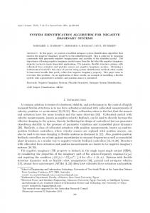
This structure is depicted in Fig. 1, where u = u 1 u 2  u p  T is the model input, M is the number of LLM neurons, and ωij denotes the LLM parameters of the ith neuron. The validity functions are chosen as normalized Gaussians; normalization is necessary for a proper interpretation of validity functions:









 1 (u1 − c i 1 )2 = exp  −  2 σ i21 

µi (u ) M

∑ µ (u )

2

2   1 (u p − c ip )  × … × exp  −  2  σ ip2  

(4)    

Fig. 1: Structure of locally linear neuro-fuzzy model

The M × P parameters of the nonlinear hidden layer are the parameters of Gaussian validity functions: center (cij) and standard deviation (σij). Optimization or learning methods are used to adjust the two sets of parameters, the rule consequent parameters of the LLMs (ωijs) and the rule premise parameters of validity functions (cijs and σijs). For further information about the LLNF models, refer to [3]. III.

RECURSIVE LEARNING METHODOLOGIES

This section is devoted to describe the recursive learning methodologies for locally liner models based on regular LoLiMoT algorithm and k-means clustering algorithm for system identification of time varying nonlinear systems. A. Tuning the premise parameters of LLNF models via a Kmeans Clustering method The regular LoLiMoT algorithm is an incremental learning algorithm and it is not possible to return to some former state during learning phase. Also, in this algorithm splitting is always done in a way that the sub-regions be equal halves. In this paper to remedy these restrictions, the k-means clustering algorithm is used in the proposed algorithm. K-means clustering minimizes the following loss function: C

N

I = ∑∑ µ ji u ( i ) − c j j =1 i =1

φi (u ) =

2 u p − c ip )      σ ip2 

( 1 (u − c ) µi (u ) = exp  −  1 2 i 1 + … +  2  σi1

2

→ min cj

(5)

where the index i runs over all elements of the sets S j , C is (3)

the number of clusters, c j are the cluster centers (prototypes)

j

j =1

737

and µ ji = 1 if the sample u ( i ) is associated (belongs) to

where Σ j is the covariance matrix of validity function j

cluster j and µ ji = 0 . The sets S j contain all indices of those

(cluster j), and c j is the cluster prototype of the cluster j,

data samples (out of all N) that belong to the cluster j, i.e., which are nearest to the cluster center c j . The cluster centers

and c i is the cluster prototype for other clusters. 4. Checking for merging clusters: this part is considered to remedy the other restriction of the regular LoLiMoT algorithm in tuning the premise parameters. After tuning the parameters of the cluster’s prototype (mean of Gaussians validity functions) and covariance matrixes, it is checked that if some clusters are close enough to merge to one cluster. This could be done by calculating the distance between cluster’s prototypes. If the distances between some clusters are smaller than a threshold which is designing parameter, these clusters is merged to a single cluster and its prototype could be calculated as follows:

c j are the parameters that the clustering technique varies in order to minimize (5). The k-means algorithm used for tuning premise parameters (validity functions) of LLNF models in the proposed method is modified to be useful for online applications. This clustering method works as follows: 1. Assigning current data sample to a proper cluster (LLM): in proposed method, the number of clusters or LLMs is not known a priori and according to the current data sample it is decided to label a new cluster to the current data sample or assign it to a proper existing cluster via some distance criteria. To do so, the minimum distance between the current data sample and the clusters’ prototype are calculated. If this value is more than a threshold which is a designing parameter, a new cluster with a prototype as current data sample is created and if it is not, current data sample is assigned to the cluster with nearest cluster prototype to the data sample. 2. Tuning the center of validity functions: If current data sample is assigned to a cluster, the centroid (mean) as the prototype of that cluster should be modified. Although, it is better to modify all the clusters’ prototype but it has to be said that such modification is a time consuming process and is not proper for online applications of this paper. The cluster prototype is modified as −

+

cj = N

N j− c j + u ( i ) N + j

− j

(6)

= N j− + 1

where u ( i ) is the current data sample, and N

j

is the

number of those data samples that belong to cluster j, and c j is the cluster’s prototype. The modification rule has a recursive form to be useful for online applications. 3. Tuning the covariance matrix of the validity functions: in this paper, the validity functions are set to be Gaussian. Therefore, the covariance matrixes of these validity functions should be tuned either. To do so, after tuning the clusters’ prototype the covariance matrix of each validity functions is set as follows:

 1 Σ j = × diag  min c j , c i  3 i≠j 

(

)

   

p

∑N cj =

(8)

i

p

N j = ∑N i i =1

The covariance matrix of this validity function (cluster) could be tuned according to 3. B. A local recursive weighted least square algorithm for tuning the consequence parts’ parameters For an online adaptation of the rule consequent parameters the local estimation approach is chosen. Therefore the numerical robustness becomes a critical issue since the number of parameters in global estimation can be very large [3]. In fact, for a large number of local linear models, global estimation cannot usually be carried out with a standard recursive least squares (RLS) algorithm [1], [19]; even numerically sophisticated algorithms can run into trouble because of the poorly conditioned problem. Assuming that the rule premises and thus the validity functions φi are known, the following local recursive weighted least squares algorithm with exponential forgetting factor can be applied separately for each rule consequent i = 1 ,…, M :

wˆ i ( k ) = wˆ i ( k − 1) + γ i ( k ) e i ( k ) , e i ( k ) = y ( k ) − u

T

( k )wˆ i ( k

1 u ( k ) P i ( k −1) + T

Pi (k ) =

738

∑N i =1

γ i (k ) =

(7)

ci

i

i =1 p

1

λi

(I −γ

i

λi

(9a)

− 1)

P i ( k −1)u ( k )

(9b)

φi ( z i ( k ) )

( k )uT ( k ) ) P i ( k −1)

(9c)

Base (NSRDB) which contains lots of weather indexes of most cities all around the world and is available online [20].

Compared with u , the augmented consequent input vector T

u = [1 x 1  x n ]

additionally contains the regressor “1” for adaptation of the offsets wi0. If prior knowledge is available, different forgetting factors λi and initial covariance matrixes P i ( 0) can be implemented for each LLM i. Fig. 2 shows the process of RLoLiMoT learning algorithm.

In this study, it is tried to predict two indexes of Kuala Lumpur city as a typical Asian city. These indexes are: 1.

Dry Bulb Temperature (degrees *10, C)

2.

Humidity Ratio (kg H2O/kg air)*104

The threshold parameter for splitting in RLoLiMoT algorithm is set to 0.3 in this case study and the threshold parameter for merging is set to 0.1. Fig. 3 shows the performance of the RLoLiMoT algorithm in one step ahead prediction of Dry Bulb Temperature index. It can be seen that in the beginning of the RLoLiMoT algorithm’s operation, the performance of the model is poor, but after a short time, the performance of the model increases rapidly. Fig. 4 shows the number of clusters during RLoLiMoT algorithm’s operation. Fig. 5 shows the performance of the RLoLiMoT algorithm in one step ahead prediction of Humidity Ratio index. It can be seen that in the beginning of the RLoLiMoT algorithm’s operation, like prediction of Dry Bulb Temperature index, the performance of the model in predicting Humidity Ratio index is poor, but after a short time, the performance of the model increases rapidly.

Fig. 3: One step ahead prediction of Dry Bulb Temperature index of Kuala Lumpur by the proposed method; (A) solid: the real index values, dashed line: prediction via RLoLiMoT algorithm; (B) one step ahead prediction error

Fig. 2: The process of RLoLiMoT algorithm.

IV.

CASE STUDIES

A. Prediction of weather indices This section is devoted to check the performance of the proposed online learning method in predicting one of the most important natural time series: weather indices because of their important role in modern human life. Most transient thermal simulations require weather data. The daily average data set has been downloaded from National Solar Radiation Data

739

Fig. 4: Number of clusters (locally linear models) during RLoLiMoT algorithm’s operation for one step ahead prediction of Dry Bulb Temperature index of Kuala Lumpur

beginning of the RLoLiMoT algorithm’s operation, the performance of the model is poor, but after a short time, the performance of the model increases rapidly. Fig. 8 shows the number of clusters during RLoLiMoT algorithm’s operation.

Fig. 5: One step ahead prediction of Humidity Ratio index of Kuala Lumpur by the proposed method; (A) solid: the real index values, dashed line: prediction via RLoLiMoT algorithm; (B) one step ahead prediction error

Fig. 6 shows the number of clusters during RLoLiMoT algorithm’s operation.

Fig. 6: Number of clusters (locally linear models) during RLoLiMoT algorithm’s operation for one step ahead prediction of Humidity ratio index of Kuala Lumpur

Fig. 7: Modeling the heat exchanger nonlinear time varying dynamics by the proposed method; (A) solid: the heat exchanger output values, dashed line: prediction via RLoLiMoT algorithm; (B) modeling error

Fig. 8: Number of clusters (locally linear models) during RLoLiMoT algorithm’s operation for modeling heat exchanger nonlinear time varying dynamics.

B. Nonlinear system identification of time varying heat exchanger dynamic This section is devoted to check the performance of the proposed online learning method in modeling a heat exchanger dynamics as a nonlinear time variant dynamics. The data set of this dynamics is available online [21]. The process is a liquid-satured steam heat exchanger, where water is heated by pressurized saturated steam through a copper tube. The output variable is the outlet liquid temperature. The input variables are the liquid flow rate, the steam temperature, and the inlet liquid temperature. In this experiment the steam temperature and the inlet liquid temperature are kept constant to their nominal values. The sampling time is one second and the number of the data is 4000. The heat exchanger process is a significant benchmark for nonlinear control design purposes, since it is characterized by a non minimum phase behavior. The threshold parameter for splitting in RLoLiMoT algorithm is set to 1.5 in this case study and the threshold parameter for merging is set to 1. Fig. 7 shows the performance of the RLoLiMoT algorithm in modeling heat exchanger nonlinear dynamics. It can be seen that in the

740

ACKNOWLEDGMENT The authors are thankful to Young Researchers Club which supports the authors of this paper during this research. V. CONCLUSIONS In this paper, the problem of online system identification of nonlinear time varying systems is considered. It has to be said that the literature on online identification methods of nonlinear system is not as rich as the literature on offline identification methods. Basically, our motivation was the possibility of using LoLiMoT algorithm as an incremental learning algorithm which has been used for modelling and control of several nonlinear systems to use its useful characteristics for tuning the parameters of LLNF models. The difficulty was the offline structure of this learning algorithm. So we had to develop this algorithm for online applications. To do so, in this paper we propose a new learning method called RLoLiMoT algorithm as an incremental learning algorithm to tune the parameters of LLNF models recursively with the aid of k-means clustering algorithm. In this algorithm some restrictions of ordinary

LoLiMoT algorithm are obviated. The performance of the LLNF models with RLoLiMoT learning algorithm is evaluated for system identification and prediction of nonlinear time variant dynamics in three case studies. Results depict the potentials of the proposed online learning method in this subject. ACKNOWLEDGMENT The authors are thankful to National Foundation of Elite which supports the authors of this paper during this research.

[8] [9] [10]

[11] [12]

REFERENCES [1] [2] [3] [4]

[5]

[6]

[7]

L. Ljung, System identification, theory for the user, Prentice-Hall, Inc. 1999. G.P. Liu, Nonlinear identification and control, a neural network approach, Springer Verlag, London, 2001. O. Nelles, Nonlinear system identification, Springer Verlag, Berlin, 2001. W. Broclanann, O. Huwendiek, “Prediction in real-time control using adaptive networks with on-line learning,” Proc. of the 3rd IEEE Conf. on Control Applications, Strathclyde University, Glasgow, pp. 1067-1072, Aug. 1994. T.W. Wan, L.C. How, “Development of feedback error learning strategies for training neurofuzzy controllers on-line,” Proc. of the 10th IEEE International Conference on Fuzzy Systems, Melbourne, Australia, pp. 1016-1021, Dec. 2001. J.A. Domínguez-Lόpez, R.I. Damper, R.M. Crowder and C. J. Harris, “Hybrid neurofuzzy online learning for optimal grasping,” Proc. of the 2nd Int. Conf. on Machine Learning and Cybernetics, Xían, 2-5 November 2003, pp. 803-808. R. Polikar, L. Udpa, S.S. Udpa, and V. Honavar, “Learn++: an incremental learning algorithm for supervised neural network,” IEEE

741

[13]

[14]

[15]

[16]

[17] [18]

[19] [20] [21]

Trans, on Systems, Man, and Cybernetics—Part C: Applications and Reviews, Vol. 31, no. 4, pp. 497-508, Nov. 2001. S. Haykin, Neural networks: a comprehensive foundation, Macmillan, New York, 1994. A. Cichoki, R. Chichester, Neural networks for optimization and signal processing, John Wiley, 1993. K.M. Bossley, Neurofuzzy modelling approaches in system identification, PhD Thesis, University of Southampton, Southampton, UK, 1997. J. Park, I.W. Sandberg, “Approximation and radial basis function networks,” Neural Comput., 5: 305-316, 1993. G. Carpenter, S. Grossberg, “The ART of adaptive pattern recognition by a self-organizing neural network,” IEEE Computer, pp. 77-88, Mar. 1988. M. Jalili-Kharaajoo, R. Ranji, and H. Bagherzadeh, “Predictive control of fossil power plant based on local linear model tree (LOLIMOT),” Proc. of IEEE, pp. 633-638, 2003. M. Jalili-Kharaajoo, A. Rahmati, and F. Rashidi, “Internal motor control based on local linear model tree (LOLIMOT) model with application to a PH neutralization process,” Proc. of IEEE, pp. 3051-3055, 2003. A. Gholipour, C. Lucas, B.N. Araabi, and M. Shafiee, “Solar activity forecast: spectral analysis and neurofuzzy prediction,” Journal of Atmospheric and Solar Terrestrial Physics, No. 67, pp. 595-603, 2005. A. Gholipour. C. Lucas, B.N. Araabi, M. Mirmomeni, M. Shafiee, “Extracting the main patterns of natural time series for long-term neurofuzzy prediction,” Neural Comput & Applications, 2006. T.A. Johansen, B.A. Foss, “NARMAX models using ARMAX models,” International Journal of Control, 58(5): 1125-1153, 1993. O. Nelles, “Local linear model tree for on-line identification of timevariant nonlinear dynamic systems” Int. Conf. on Artificial Neural Networks (ICANN), Bochum, Germany, pp. 115-120, July 1996. R. Iserman, Identifikation dynamischer systeme – Band 1, 2. ed. Springer, Berlin, 1992. http://sel.me.wisc.edu/trnsys/weather/weather.htm. http://homes.esat.kuleuven.be/~smc/daisy.