We propose here one way, called Bootstrap, to do it using computer intensive
techniques ... Originally, the Bootstrap was introduced to compute standard error
of.
Introduction to resampling methods
Introduction We want to assess the accuracy (bias, standard error, etc.) of an arbitrary estimate θˆ knowing only one sample x = (x1 , · · · , xn ) drawn from an unknown population density function f .
Definitions and Problems
We propose here one way, called Bootstrap, to do it using computer intensive techniques for resampling.
Non-Parametric Bootstrap Parametric Bootstrap
Bootstrap is a data based simulation method for statistical inference. The basic idea of bootstrap is to use the sample data to compute a statistic and to estimate its sampling distribution, without any model assumption.
Jackknife Permutation tests Cross-validation
No theoretical calculations of standard errors needed so we don’t care how mathematically complex the estimator θˆ can be!
25 / 133
Introduction
26 / 133
Bootstrap samples and replications
The (non-parametric) bootstrap method is an application of the plug-in principle. By non-parametric, we mean that only x is known (observed) and no prior knowledge on the population density function f is available. Originally, the Bootstrap was introduced to compute standard error of an arbitrary estimator by Efron (1979) and to-date the basic idea remains the same. The term bootstrap derives from the phrase to pull oneself up by one’s bootstrap (Adventures of Baron Munchausen, by Rudolph Erich Raspe). The Baron had fallen to the bottom of a deep lake. Just when it looked like all was lost, he thought to pick himself up by his own bootstraps.
27 / 133
Definition A bootstrap sample x∗ = (x1∗ , x2∗ , · · · , xn∗ ) is obtained by randomly sampling n times, with replacement, from the original data points x = (x1 , x2 , · · · , xn ). Considering a sample x = (x1 , x2 , x3 , x4 , x5 ), some bootstrap samples can be: x∗(1) = (x2 , x3 , x5 , x4 , x5 ) x∗(2) = (x1 , x3 , x1 , x4 , x5 ) etc.
Definition With each bootstrap sample x∗(1) to x∗(B) , we can compute a bootstrap replication θˆ∗ (b) = s(x∗(b) ) using the plug-in principle. 28 / 133
How to compute Bootstrap samples
How many values are left out of a bootstrap resample ?
Repeat B times:
Given a sample x = (x1 , x2 , · · · , xn ) and assuming that all xi are different, the probability that a particular value xi is left out of a resample x∗ = (x1∗ , x2∗ , · · · , xn∗ ) is: � � 1 n ∗ P(xj 6= xi , 1 6 j 6 n) = 1 − n �n since P(xj∗ = xi ) = n1 . When n is large, the probability 1 − n1 converges to e −1 ≈ 0.37.
1
A random number device selects integers i1 , · · · , in each of which equals any value between 1 and n with probability n1 .
2
Then compute x∗ = (xi1 , · · · , xin ).
Some matlab code available on the web See BOOTSTRAP MATLAB TOOLBOX, by Abdelhak M. Zoubir and D. Robert Iskander, http://www.csp.curtin.edu.au/downloads/bootstrap toolbox.html
29 / 133
30 / 133
The Bootstrap algorithm for Estimating standard errors
Bootstrap estimate of the standard Error Example A
1
Select B independent bootstrap samples from x
2
Evaluate the bootstrap replications: θˆ∗ (b) = s(x∗(b) ),
3
x∗(1) , x∗(2) , · · ·
, x∗(B)
drawn
From the distribution f : f (x) = 0.2 N(µ=1,σ=2) + 0.8 N(µ=6,σ=1). We draw the sample x = (x1 , · · · , x100 ) : 7.0411 5.2546 7.4199 4.1230 3.6790 −3.8635 −0.1864 −1.0138 6.9523 6.5975 x= 6.1559 4.5010 5.5741 6.6439 6.0919 7.3199 5.3602 7.0912 4.9585 4.7654
∀b ∈ {1, · · · , B}
ˆ by the standard deviation of the B Estimate the standard error sef (θ) replications: "P #1 B ˆ∗ ˆ∗ 2 2 b=1 [θ (b) − θ (·)] se ˆB = B −1 where θˆ∗ (·) =
PB
ˆ ∗ (b) θ B
b=1
4.8397 7.3937 5.3677 3.8914 0.3509 2.5731 2.7004 4.9794 5.3073 6.3495 5.8950 4.7860 5.5139 4.5224 7.1912 5.1305 6.4120 7.0766 5.9042 6.4668
5.3156 4.3376 6.7028 5.2323 1.4197 −0.7367 2.1487 0.1518 4.7191 7.2762 5.7591 5.4382 5.8869 5.5028 6.4181 6.8719 6.0721 5.9750 5.9273 6.1983
6.7719 4.4010 6.2003 5.5942 1.7585 0.5627 2.3513 2.8683 5.4374 5.9453 5.2173 4.8893 7.2756 4.5672 7.2248 5.2686 5.2740 6.6091 6.5762 4.3450
7.0616 5.1724 7.5707 7.1479 2.4476 1.6379 1.4833 1.6269 4.6108 4.6993 4.9980 7.2940 5.8449 5.8718 8.4153 5.8055 7.2329 7.2135 5.3702 5.3261
We have µf = 5 and x = 4.9970. 31 / 133
Bootstrap estimate of the standard Error
32 / 133
Distribution of θˆ
1
B = 1000 bootstrap samples {x∗(b) }
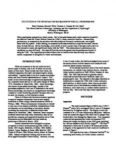
When enough bootstrap resamples have been generated, not only the standard error but any aspect of the distribution of the estimator θˆ = t(fˆ) could be estimated. One can draw a histogram of the distribution of θˆ by using the observed θˆ∗ (b), b = 1, · · · , B.
2
B = 1000 replications {x ∗ (b)}
Example A
3
Bootstrap estimate of the standard error:
Example A
se b B=1000 =
"P
1000 ∗ b=1 [x (b)
x ∗ (·)]2
− 1000 − 1
350
# 12
300
250
= 0.2212
200
150
where x ∗ (·) = 5.0007. This is to compare with se(x) ˆ =
ˆ σ √ n
= 0.22.
100
50
0
0
2
4
5
6
8
10
Figure: Histogram of the replications {x ∗ (b)}b=1···B . 33 / 133
Bootstrap estimate of the standard error
34 / 133
Bootstrap estimate of the standard Error
How many B in practice ? you may want to limit the computation time. In practice, you get a good estimation of the standard error for B in between 50 and 200.
Definition The ideal bootstrap estimate sefˆ (θˆ∗ ) is defined as:
Example A
lim se ˆ B = sefˆ (θˆ∗ )
B→∞
sefˆ
(θˆ∗ )
is called a non-parametric bootstrap estimate of the standard error.
B se bB
10 0.1386
20 0.2188
50 0.2245
100 0.2142
500 0.2248
1000 0.2212
10000 0.2187
Table: Bootstrap standard error w.r.t. the number B of bootstrap samples.
35 / 133
36 / 133
Bootstrap estimate of bias
Bootstrap estimate of bias
Definition
1
B independent bootstrap samples x∗(1) , x∗(2) , · · · , x∗(B) drawn from x
2
Evaluate the bootstrap replications:
The bootstrap estimate of bias is defined to be the estimate: ˆ = Eˆ [s(x∗ )] − t(fˆ) Biasfˆ (θ) f
θˆ∗ (b) = s(x∗(b) ),
= θˆ∗ (·) − θˆ 3
Approximate the bootstrap expectation :
Example A B Efˆ (x ∗ ) d Bias
10 5.0587 0.0617
20 4.9551 -0.0419
50 5.0244 0.0274
100 4.9883 -0.0087
500 4.9945 -0.0025
1000 5.0035 0.0064
B B 1 X ˆ∗ 1 X θˆ∗ (·) = θ (b) = s(x∗(b) ) B B
10000 4.9996 0.0025
b=1
4
d of x ∗ (x = 4.997 and µf = 5). Table: Bias
∀b ∈ {1, · · · , B}
b=1
the bootstrap estimate of bias based on B replications is: d B = θˆ∗ (·) − θˆ Bias
37 / 133
Confidence interval
38 / 133
Can the bootstrap answer other questions?
The mouse data Definition Using the bootstrap estimation of the standard error, the 100(1 − 2α)% confidence interval is: θ = θˆ ± z (1−α) · se bB
Data (Treatment group)
94; 197; 16; 38; 99; 141; 23
Data (Control group)
52; 104; 146; 10; 51; 30; 40; 27; 46
Definition
If the bias in not null, the bias corrected confidence interval is defined by: d B ) ± z (1−α) · se θ = (θˆ − Bias bB
Table: The mouse data [Efron]. 16 mice divided assigned to a treatment group (7) or a control group (9). Survival in days following a test surgery. Did the treatment prolong survival ?
39 / 133
Can the bootstrap answer other questions?
The Law school example
The mouse data Remember in the first lecture, we compute d = x Treat − x Cont = 30.63 with a standard error se(d) ˆ = 28.93. The ratio was d/se(d) ˆ = 1.05 (an insignificant result as measuring d = 0 is likely possible). Using bootstrap method 1
2 3
4
∗(b)
∗(b)
40 / 133
∗(b)
B bootstrap samples xTreat = (xTreat 1 , · · · , xTreat 7 ) and ∗(b) ∗(b) ∗(b) xCont = (xCont 1 , · · · , xCont 9 ), ∀1 6 b 6 B ∗(b) ∗(b) B bootstrap replications are computed: d ∗ (b) = x Treat − x Cont The bootstrap standard error is computed for B = 1400: se ˆ B=1400 = 26.85. The ratio is d/se ˆ 1400 (d) = 1.14.
School LSAT (X) GPA (Y)
1 576 3.39
2 635 3.30
3 558 2.81
4 578 3.03
5 666 3.44
6 580 3.07
7 555 3.00
School LSAT (X) GPA (Y)
9 651 3.36
10 605 3.13
11 653 3.12
12 575 2.74
13 545 2.76
14 572 2.88
15 594 2.96
8 661 3.43
Table: Results of law schools admission practice for the LSAT and GPA tests. It is believed that these scores are highly correlated. Compute the correlation and its standard error.
This is still not a significant result.
41 / 133
42 / 133
Correlation
The Law school example
The estimated correlation is corr(x, d y) = .7764 between LSAT and GPA.
The correlation is defined : corr(X , Y ) =
E[(X − E(X )) · (Y − E(Y ))]
(E[(X − E(X ))2 ] · E[(Y − E(Y ))2 ])1/2
Non-parametric Bootstrap estimate of the standard error B se ˆB
Its typical estimator is: Pn −n x y i=1 xi yi P corr(x, d y) = Pn 2 2 1/2 [ i=1 xi − nx ] · [ ni=1 yi2 − ny 2 ]1/2
25 .140
50 .142
100 .151
200 .143
400 .141
800 .137
1600 .133
3200 .132
Table: Bootstrap estimate of standard error for corr(x, d y) = .776.
d ≈ .132. The standard error stabilizes to sefˆ (corr)
43 / 133
The Law school example: Conclusion
44 / 133
Summary
Re-sampling of x to compute bootstrap samples x∗
The textbook formula for the correlation coefficient is: √ se( ˆ corr) d = (1 − corr d 2 )/ n − 3
With corr d = 0.7764, the standard error is se( ˆ corr) d = 0.1147.
The estimated non-parametric bootstrap standard error seB=3200 is 0.132.
45 / 133
Computation of bootstrap replication of the estimator θˆ∗ (b) for b = 1, · · · , B d B and the From replications, standard error se b B , the bias Bias confidence interval. Non-parametric bootstrap estimations (no prior on f ).
46 / 133