intrusion detection using bayesian classifier for arbitrarily long ... - iadis

IADIS International Journal on Computer Science and Information Systems Vol. 9, No. 1, pp. 71-81 ISSN: 1646-3692

INTRUSION DETECTION USING BAYESIAN CLASSIFIER FOR ARBITRARILY LONG SYSTEM CALL SEQUENCES Nasser Assem. Al Akhawayn University, Ifrane 53000, Morocco. [email protected]

Tajjeeddine Rachidi. Al Akhawayn University, Ifrane 53000, Morocco. [email protected]

Mohamed Taha El Graini. Al Akhawayn University, Ifrane 53000, Morocco. [email protected]

ABSTRACT In this paper, we present a sequence classifier for detecting host intrusions from long process system call sequences. The proposed classifier (called SC2.2) is a naïve Bayes classifier that builds class conditional probabilities from Markov modeling of system call sequences. We describe the proposed classifier, and then provide experimental results on the widely used University of New Mexico’s system call trace data sets. The results of our proposed classifier are benchmarked against leading classifiers, namely naive Bayes multinomial, C4.5 decision tree, RIPPER, support vector machine, and logistic regression. A key feature of the proposed classifier is its ability to handle efficiently arbitrarily long sequences, and zero transitional probabilities in the modeled Markov chain, by using a ―test, backtrack, scale and remultiply‖ technique, and using the m-estimate of conditional probabilities. Furthermore, it capitalizes on IEEE standard for floating-point arithmetic error specification to return classification confidence. Results show that the proposed classifier yields a better performance than standard classifiers on most datasets used. KEYWORDS

Intrusion detection, System call sequence, Naive Bayes classifier, Markov model, M-estimate

1. INTRODUCTION An intrusion detection system gathers and analyzes traces from various areas within a computer or a network to identify possible security breaches (Patcha, 2007). In other words, intrusion detection is the act of detecting actions that attempt to compromise the confidentiality, integrity or availability of a system/network. Traditionally, intrusion detection systems have been classified as: signature detection systems, anomaly detection systems or hybrid/compound detection systems, combining both techniques (Patcha, 2007). A signature detection system identifies pre-established patterns of traffic or application activity presumed to be malicious. This type of detection is commonly found in network intrusion detection systems (NIDS). Therein, signatures range from very simple – checking the value of various TCP/IP headers fields – to highly complex signatures that may require deep packet inspection (Thinh, 2012) techniques involving the application layer payload and/or tracking the state of a connection, and/or performing extensive protocol analysis. Signatures are written in a proprietary language, and stored in a signature database that is updated periodically. Signature-based NIDS scan every IP datagram for known signatures in the signature database. An attack is declared when a match occurs. NIDS are widely available in the market in the form of standalone appliances or software, and are often placed at the entry/frontier of the network in collocation with firewalls, as well as, within the internal network itself in locations where they capture all/most of the traffic. This said, as TCP/IP traffic explodes exponentially, NIDS suffer from real scalability challenges, namely the ability to perform signature matching for tens of thousands known intrusions against tens of thousands, if not hundreds of thousands, simultaneous connections at wire speed, so as not to introduce delays in connections. Furthermore, the number of attacks is

71

also increasing drastically and the ability to produce signatures rapidly, so as to counter zero-day1 vulnerabilities is not always possible. Not to mention the inability to perform deep packet inspection on the increasingly encrypted traffic (IPv6 encrypts traffic by default), and that a great deal of attacks/intrusions are nowadays carried out via application layer, such as XSS, against which NIDS are not effectives (Du, n.d.). Anomaly detection systems, on the other hand, compare activity (network traffic or application activity within a host) against a normal baseline behavior also called profile. This type of intrusion detection is pertinent to both NIDS and to host intrusion detection systems (HIDS). In HIDS, an anomaly is defined as a pattern that does not conform to expected normal behavior/profile. A straightforward anomaly detection approach consists in defining a profile of activity on a host/computer representing normal behavior, and declaring patterns which do not fit to the normal profile, in the logged observations, as an anomaly/intrusion. Like signature IDSs, many challenges are often encountered when dealing with anomaly detection, namely (i) defining a normal profile of application activity that caters for every possible normal behavior is difficult, and the boundaries between normal and anomalous behaviors are often blurred: an observation which lies close to the boundary can equally be labeled normal and intrusive; (ii) often too, malicious adversaries, like viruses and worms adapt their intrusion patterns to make the anomalous observations appear like normal, thereby making the task of defining normal behavior more challenging; (iii) normal behavior keeps evolving and a current notion of normal behavior might not be sufficiently representative in the future; and finally (iv) building the normal profile requires adaptive learning techniques which require a great deal of data that must be collected beforehand. Machine learning techniques in general and data mining techniques in particular (Eskin, 2001; Chebrolu, 2005; Syed, 2009; Nadiammai, 2011; Rao, 2011, Riad, 2011; Chandola, 2012) have been used to classify program behavior, and to detect intrusions based on pattern/profile discovery. Despite these shortcomings, HIDS represent the way forward in dealing with intrusion, and the most investigated HIDS approach is system call analysis; that is, inspection of the requests made by a user program (which may or may not be intrusive) to the operating system. The pattern of these requests is believed to be a good discriminator between normal and abnormal behavior of a program, thus giving indications as to the possibility of an attack. Indeed, the life cycle of an infected/intruding program consists in major phases: discovery, replication (pro-creation), disguise, and assault, leading to the execution of series of system calls such as, repeated scan of the network, access to the file system and/or boot sector, spawning of offspring etc.), which a normal productive user program does not normally do. Intrusion detection from system calls offers a way to circumvent the encryption challenge for NIDS, since it gives access to data (probably as parameters to system calls) after the standard decryption mechanisms take place in the destination host kernel protocol stack. It is also the way forward in the convergence between NIDS and HIDS and in coping with the exponential number of threats. At the heart of system call–based intrusion detection is capturing sequences of system calls and their input and output. One such tool that offers capturing capabilities is Sebek (Anon., 2003). Sebek captures intrusion activities on a host (typically a honeypot), without the attacker (hopefully) knowing it. The captured data include system call ID and its input and output parameters. The capture of input and output information opens new venues for intrusion detection and prevention, as it allows for further profiling of intrusive behavior through the sequence of data used by system calls invoked by an intrusive process/program. Although, captured system calls and their parameters do not yield information on attacks guided towards the operating system itself or its protocol stacks (IP/TCP…), we believe that Sebek, if extended to capture system call parameters other than the currently read() and write(), will help extend the research on HIDS and NIDS in a unified way, and explore better anomaly detection mechanisms, capitalizing on the huge amounts of activity traces that can be captured.

2. RELATED WORK Forrest (1996) introduced one of the earliest methodologies that involved analyzing a program’s system call sequences, and showed that correlations in fixed length sequences of system calls could be used to build a normal profile of a program. Programs that show sequences that deviated from the normal sequence profile could then be considered to be victims of an attack, such as an infection by a virus or a worm. The system uses previously collected data packed in a simple table-lookup algorithm to learn the profiles of programs (Patcha, 2007). Despite many shortcomings, this initial work was extended by many, including (Warrender, 1999), (Wagner, 2001), (Feng, 2003), (Hu, 2009), and (Hoang, 2009). To date, system call based sequence analysis remains the most popular choice for analyzing program behavior. From a modeling perspective, Markov modeling has been used extensively to detect probable (sub)sequences of intrusion in system calls (Hu, 2009) and (Hoang, 2004). These computationally very expensive 1

A vulnerability that comes to be known right after shipment of software and before software editor has had the time to address it.

72

approaches consist in two slow convergence processes, one for training the hidden Markov model that fits best an observed sub-sequence, obtained by minimizing the conditional probability of a sub-sequence given the previous hidden Markov model (Baum-Welch algorithm) (Rabiner, 1989); and another one for combining, using weighted addition, the hidden Markov models obtained for different sub-sequences into one final global Markov model. There have been several suggestions to improve the performance of HMM-based Intrusion detection methods, such as multi HMM and multi-layer HMM (Kang, 2005). More discussions were concerned with training the model suggesting offline training, machine learning approaches, or using sub-HMM, where the training dataset is divided into subsets of sequences used for training the sub HMM models, and finally aggregating the sub models to get the final model. Wang (2010) summarizes different HMM based models along with their strengths and weaknesses. Apart from their slowness, various deficiencies are inherent to HMM-based techniques: Most notably is the fact that there is no proof that the final model i.e., combination of models obtained from disjoint sub-sequences yields a model that caters of long sequences; An obvious avoidance mechanism consists of designing a sequence that is unsafe/intrusive, and yet its sub-sequences are all safe/non-intrusive. Furthermore, the learning has been made out of normal sequences exclusively2. The underlying assumption is that all that is not normal is intrusive. This strict two class classification does not portrait reality where various levels of threat are needed to guide the decision of network administrators to appropriate action. The use of a threshold and different sub-sequence lengths (23 and 35) for different datasets is an indication of the absence of a sequence length that yields acceptable performance across various datasets. This makes the whole approach very specific to the dataset underhand. More recently, techniques for detecting illegal system calls based on a data-oriented model have emerged (Demay, 2011 and Nidhra, 2012). Contrary to classical system call analysis models, where an intrusion is detected when deviations from the normal control flow of the system based on its system calls sequences is detected, the aim of data-oriented models try to detect attacks against the integrity of the systems calls themselves, or attacks in which the intruder mimics the normal behavior of the program, but still passes rogue data that may lead to intrusion. This approach certainly adds a second perspective to system call analysis for proper control flow, i.e., the analysis of application data objects at run time. ElGraini (2012) presented a technique for system call sequence classification that combines naive Bayes approach with Markov chain modeling for sequence classification. Specifically, it builds separate Markov models for normal and intrusive sequences from very long sequences of system calls. These models are then used to classify sequences of system calls into two classes: normal or intrusive. The technique uses first order observable Markov model rather than a hidden Markov model on the one hand, and classification of sequences of any length through naïve Bayes classifier. The two Markov models are built separately for intrusive and normal sequences, with the classifier allowing for a grey zone classification. However, this approach suffers from the problems posed by zero-transitional probabilities in the Markov chain probability matrix, thus yielding inaccurate classification results. In this paper we aim to overcome this deficiency by (i) introducing the technique of m-estimate of class conditional probabilities (Tan, 2006, pp. 236 – 237) to address the issue of posterior probabilities becoming zero as soon as a transition probability is zero, and (ii) performing extensive testing that yields the optimal value for the parameters of the m-estimate technique. Sections below give details of the procedure for building the classification model, the use of m-estimate of class conditional probabilities, and the adaptation of BSR algorithm for handling very low probabilities.

3. MODELING AND LEARNING Our proposed classifier classifies arbitrarily long sequences of system calls made by a process, using a naïve Bayes classification approach, with class conditional probabilities derived from Markov chain modeling of sequences. In the following sections, we give more details about (i) naïve Bayes classification; (ii) Markov models; (iii) how the two concepts are combined to classify system call sequences; and (iv) an example that illustrates such classification.

3.1 Naïve Bayes Classifier

2

Strictly speaking, learning from the positive class is a signature finding rather than classification

73

Formally, let s = (s1, s2,… sn) be a test sequence made of system calls s1, s2, …, sn. The classification consists in finding the class c with the highest posterior probability given the sequence s. Based on Bayes theorem, the posterior probability of class c given sequence s is: P(

)

P(

)

P( )

P(

)



where S and C are random variables denoting sequences and classes, P(S = s |C = c) is the class conditional probability of sequence s given class c. P(C = c) is the prior probability of class c, and P(S = s) is the prior probability of sequence s. Since P(S = s) is independent of the class, the task of classifying s becomes then to maximize the posterior probability, i.e., ()

argmaxc P(

)

P(

)

We define class 0 to be the class of normal sequences, and class 1 to be the class of intrusive sequences. Like in naïve Bayes classifier, we estimate the class conditional probability of sequence s and the prior probability of class c from the training data (learning). The prior probabilities P(C = 0) and P(C = 1) of classes 0 and 1 are estimated from the training data set respectively as the fraction of training sequences labeled class 0 and 1, using Markov model to estimate the class conditional probabilities of a sequence s.

3.2 Observable Markov Chain Model An observable Markov process is a system where the dynamics can be modeled as a process that moves from state to state depending (only) on the previous n states. The process is called an order n model where n is the number of states affecting the choice of next state. In a first order process with M states, there are M2 transitions between states, since it is possible for any one state to follow another. Associated with each transition is a probability called the state transition probability - this is the probability of moving from one state to another. The M2 transition probabilities are regrouped into a transition matrix TP. The initial probabilities for each state are also regrouped into a vector called the initial probability vector (IP). In trying to recognize patterns in time as is the case with system call sequences, discrete time steps and discrete states, are used. With these assumptions, the system producing the sequences of system calls can be described as a Markov process consisting of an IP vector and a state transition matrix TP. An important point about the assumption is that the state transition probabilities do not vary in time - the matrix is fixed throughout the life of the system. With this, each call causes the system to change state (possibly back to the same state). This is an observable Markov model since the output of the process is the set of states at each instant of time, where each state corresponds to a system call (observation). Formally, we model a sequence s = (s1, s2,…, sn) as a Markov chain where its occurrence probability in class c is estimated as: P ( n 1 2 … n-1 ) P ( 1 ) P (s1 , 2 ) … P ( n-1 , n ), (3) where Pc(s1) is the initial probability of system call s1, and Pc(si, sj) is the probability of system call sj is invoked after system call si is invoked in class c. The class conditional probability of sequence s given class c is, then, estimated from the training data as: | P( ) P ( 1 ) P ( 1 , 2 ) … P ( n-1 , n ), (4) where Pc(s1) is the initial probability of system call s1, and Pc(si, sj) is the transition probability Pc(si, sj) estimated from the training data for both normal data (C = 0) set and intrusive data (C = 1). For this purpose, during the training phase, we build for each class c: (i) the initial count vector ICc, where ICc[i] is the count of sequences of class c that start with system call i, and (ii) the transition count matrix TCc, where TCc[i, j] is the count of instances where system call j is invoked after system call i. We then compute the initial probability vector IPc, where IPc[i] is the probability that a sequence of class c starts with system call i, estimated as the fraction: IC

IP

(5)

j ICc

and the transition probability matrix Tc, where Tc[i, j] is the probability of system call j following i, estimated as the fraction: TCc

TP ,

k TCc

, ,

(6)

3.3 Classification The classification of a sequence s, given the learned normal and intrusive classes, consists in finding the class that maximizes the posterior probability of that class as in equation (2). If, however, the classes have equal posterior probabilities (grey zone), then one can either accept a non-classification of the sequence, or use the class prior probabilities to break ties. In most binary classification cases, the normal class is the majority class 74

since usually there are more normal instances than anomalous ones in the raining data sets. In our case, we have used the latter strategy, i.e., used the majority class (normal) to resolve grey zone issues, because an intrusion detection system has to decide whether to stop the activity (assuming it is intrusive) to avoid any damage, or let it finish (assuming it is normal). This policy is not built into the classification modeling and can be set differently by a system administrator. The following example illustrates the model.

3.4 Example Without loss of generality, we assume that the system has only three system calls: a, b and c. For the training data, we use the sequences: s00 = (a, b, c), s01 = (b, b, c), s02 = (a, c, b) labeled as normal, and s10 = (a, a, a) and s11 = (c, c, b) labeled as intrusive. From this training data set, we produce the initial probability vectors the two classes (IP0 and IP1), and the transition probability matrices for the two classes (TP0 and TP1): [ ] IPo [2/3 1/3 0] [

]

[

]

Consider the following test sequence s = (c, c, c) to be classified. We compute:  The class conditional probability of s given class 0 is P(S = s | C = 0) = P0(c) × P0(c|c) × P0(c|c), where the probability that a sequence starts with a c given class 0 is P0(c) = 0, and the probability that system call c follows itself in a sequence of class 0 is P0(c|c) = 0. So, P(S = s | C = 0) = 0.  The class conditional probability of s given class 1 is P(S = s | C = 1) = P1(c) × P1(c|c) × P1(c|c), where the probability that a sequence starts with a c given class 1 is P1(c) = 1/2, and the probability that system call c follows itself in a sequence of class 1 is P1(c|c) = 1/2. So, P(S = s | C = 1) = 1/8. Since the prior probability of the normal class is P(C = 0) = 3/5, and the prior probability of the intrusive class is P(C = 1) = 2/5, then the posterior probability of class 1 is P(S = s | C = 1) × P(C = 1) = 1/20 and is greater than that of class 0, which is P(S = s | C = 0) × P(C = 0) = 0. Therefore, the test sequence s is classified as intrusive (class 1). The example provided above is simple, and the sequences used are significantly shorter than real samples. In the data sets that we used, the number of different system calls is 182 and sequences can grow as large as 183,018 system calls (as is the case of sendmail synthetic data set of UNM). The calculations of the class conditional probabilities P(S = s | C = c) entail multiplying as many as thousands of times transition probabilities. This can lead to hugely small numbers/errors because of granularity of floating point calculations on most computers, yielding classification errors (both posterior probabilities for class 0 and 1 will be zero).

4. IMPLEMENTATION ISSUES A few implementation issues have an impact on the quality (accuracy, detection rate etc.) of naïve Bayes-like classifiers that use Markov modeling. Chief among these are the impact of zero conditional probabilities, and the product of a very large number of probabilities. In the following subsections, we address the main implementation issues.

4.1 Handling Zero Transitional Probabilities This section addresses the issue of a zero transition probability that causes a whole conditional probability to vanish (to zero). The pseudo-counts as proposed in (Krogh, 1998), where all the counts are augmented by one does not yield better results than original SC2. We are using the m-estimate (Tan, 2006), where the probability of transition (i, j) is estimated as: [

[ ]

]

[

]

(7)

where m is the equivalent sample size and p is the estimated prior probability of transition (i, j). One needs to estimate m and p for a given classifier. In our case, since the sum of all transitional probabilities starting at system call i is 1, as can be noticed in equation (6) and as is assumed in a Markov chain in general, we can deduce that p should be equal to 1/Im, where Im is the number of different system calls (182 in our case). A similar estimation can be used for initial probability vectors. As for the other parameter in equation (7), an optimal value for the equivalent sample size (m) can be identified by varying m, generating multiple candidate classifiers, and choosing the one model (optimal) with better accuracy and detection rate.

75

If we use m-estimate with m=1and p=1/3 in the example of section 3.4 (above), then the initial probability vectors and transition probability matrices become: ] [ ] IPo [ /12 4/12 [

]

[

]

4.2 Test, Backtrack, Scale and Re-multiply (TBSR) While computing class conditional probabilities of a sequence, if the sequence is relatively long, the latter may become too small to be represented with a normal floating-point real number. For example, the longest sequence of sendmail (UNM) is composed of 183,018 system calls. The product of transition probabilities can get very small quickly especially when those probabilities are themselves very small. The values become too small to be represented by any machine. To avoid subnormal values, and also to avoid the cumulative effect of gradual underflow of floating-point multiplications by very small real numbers, we backtrack whenever a class conditional probability becomes less than the smallest normal positive number LDBL_MIN = 3.36 × 104932 (Anon., 2008), scale it by the largest number LDBL_MAX = 1.19 × 104932, and re-multiply by the transition probability. The number of times the scaling is applied is recorded to be used for final comparison of posterior probabilities of classes 0 and 1. In what follows, we give the TBSR algorithm (adapted to use m-estimate), since conditional probabilities do not get null.

4.2.1 TBSR Algorithm Let P = p1 × p2 … × pk a product of class conditional probabilities representing the transitional probabilities corresponding to a sequence of k system calls. P can be computed as M × LDBL_MAX E, |E| is the number of times the scaling up took place to avoid subnormal values, and M the corresponding representable value. FUNCTION TBSR(p1, p2,…, pk)RETURNS STRUCT (long double M, long double E) // p1, p2,…, pk: sequence of probabilities // P = M x LDBL_MAXE, |E| is the # of times scaling was performed // M the corresponding representable value (between LDBL_MIN and LDBL_MAX) BEGIN DECLARE P STRUCT (long double M, long double E); P.M = p1; P.E = 0; FOR i = 2 TO k DO temp = P.M; P.M = P.M * pi; IF (P.M < LDBL_MIN) THEN // subnormal value: backtrack and scale P.M = temp * LDBL_MAX; P.M = P.M * pi; /* re-multiply */ P.E = P.E - 1; /* update exponent (# of scaling) */ ENDIF ENDFOR RETURN P; END

TBSR() can be invoked for the purpose of classification as follows: FUNCTION CLASSIFY(s, IP0, TP0, IP1, TP1) RETURNS INT /* class 0 or 1 */ // s: sequence of system calls to be classified // IP0, IP1: Initial probability vectors from Markov model (for C0 and C1) // TP0, TP1: Transitional probability matrices from Markov model BEGIN // Get the class conditional probabilities of s for classes 0 and 1: (M0,E0) = TBSR(IP0[s[1]],TP0[s[1], s[2]],…,TP0[s[len(s)-1], s[len(s)]); (M1,E1) = TBSR(IP1[s[1]],TP1[s[1], s[2]],…,TP1[s[len(s)-1], s[len(s)]); // Compute posterior probabilities of C0 and C1 M0 = M0 * prior[0]; M1 = M1 * prior[1]; IF (E1 > E0) RETURN 1 // scaled more times => smaller ELSE IF (E1 < E0) RETURN 0 ELSE IF (M1 < M0) RETURN 0 ELSE IF (M1 > M0) RETURN 1 ELSE RETURN 1 // Tie: flag as intrusive C1 to be safe END

4.2.2 Advantages of TBSR

76

While it would be possible to use logarithms, we preferred to use TBSR and took relative error into account to get around the significant obstacle of computing class probabilities of long sequences. It is to be noted that the implementation of logarithm functions (Hoang, 2004 and Rabiner, 1989) differ depending on compiler/libraries and bounds on errors are not always provided for specific implementations which may entail unnecessary scaling, because of uncertainty introduced by the log computations itself, and thus more computation time. This very effective approach allowed us to avoid cumbersome techniques that consist in training with series of Markov models with limited sub-sequences as in (Hu, 2009). The effect of this technique greatly reduces the time complexity of the learning phase, as shall be shown in the results’ section.

4.3 Calculation Error Considerations When comparing class posterior probabilities using TBSR algorithm, relative error estimation is used when comparing posterior probabilities of class ± (1+Ɛ) len(seq), where Ɛ is given for floating-point operations as 1.08 × 10-19 (Anon., 2008).

5. EXPERIMENTS To benchmark our proposed classifier (SC2.2), we used data sets from a public database (Forrest., n.d.) provided by the University of New Mexico (UNM), and the Massachusetts Institute of Technology (MIT) Artificial Intelligence Laboratory. They contain traces from sendmail - the most popular UNIX-based implementation of the Simple Mail Transfer Protocol (SMTP) for transmitting emails in UNIX systems and lpr -UNIX program tool for sending print jobs to printers: print server- processes, which are major applications commonly and extensively invoked in Unix based computing environments. Sendmail dataset — the synthetic sendmail is the main dataset. The sendmail intrusive data were collected at UNM on Sun SPARC stations running unpatched SunOS 4.1.1 and 4.1.4 and sendmail daemon subject to syslogd intrusion. The syslogd attack exploits buffer overflow vulnerability in sendmail, causing the replacement of part of endma l’ running image with the attacker’s machine code. The intrusive code is then executed, yielding a forked root-owned shell listening to a port. The attacker may then attaches to this port remotely. UNM lpr dataset — the intrusive data for lpr were collected on Sun SPARC stations running unpatched SunOS 4.1.4 with the lpr program subject to lprcp intrusion attack. The lprcp attack script uses lpr to replace the contents of an arbitrary file with others. The attack exploits the fact that this version of lpr uses only 1000 different names for printer queue files, and do not remove the old queue files before resuming them. The attack produces 1001 traces. In the first trace lpr places a symbolic link to the victim file in the queue. The subsequent traces advance lpr’ counter, until on the last trace the victim file can be overwritten with the attacker’s own material. Trace files contain pairs of process ID and ID of system call made by that process. Multiple processes can appear in the same file. Hence, we grouped them by process ID to generate a sequence per process in each trace. Table 1 gives the summary of the data sets used, as provided by the university of New Mexico (Kang 2005, Forrest., n.d.): Table 1. The number of original traces and generated sequences in UNM data sets Program synthetic sendmail (normal) synthetic sendmail (exploit) synthetic sendmail CERT (normal) synthetic sendmail CERT (exploit) live lpr (normal) live lpr (exploit) live lpr MIT (normal) live lpr MIT (exploit)

# of sequences 346 25 294 34 1,231 1,001 2,697 1,001

Max length 183,018 1,002 182,901 919 39,306 188 59,565 189

Avg length 5202 270 5361 245 450 164 1080 165

In order to make sure that no training data are used for testing, the 10-fold cross validation method (Kang, 2005) was used. In other words, from the traces of the data sets, we generate 10 equal sized sub data sets that have each a number of intrusive sequences and a number of normal sequences proportional to the global data set. One of the subsets is picked for testing and the remaining 9 are used for learning. This is repeated over all the 10folds. The counts of correctly (or incorrectly) classified sequences are added over all the folds to assess the performance of the overall classification model. The performance of our classifier is assessed and compared to other techniques in the next section.

77

6. RESULTS To assess the performance of our classifier, the numbers of test sequences (not used in training) correctly and incorrectly classified by the system are counted. If we refer to the normal sequences (majority class) as ―negative‖, and the intrusion sequences as ―positive‖, then the following are computed: (i) TP (true positives): the number of intrusive sequences correctly classified; (ii) FN (false negatives): the number of intrusive sequences incorrectly classified; (iii) TN (true negatives): the number of normal sequences correctly classified; and (iv) FP (false positives): the number of normal sequences incorrectly classified. Table 2 represents those counts as a confusion matrix (Patcha, 2007, and Tan, 2006): Table 2. Possible results of intrusion detection systems predicted class intrusive normal actual class

intrusive

TP

FN

normal

FP

TN

The performance of a classifier can be measured with a few metrics: (i) accuracy: the fraction of input sequences predicted correctly; (ii) detection rate: the fraction of intrusive sequences predicted correctly; and (iii) false positive rate (FPR): the fraction of normal sequences predicted as intrusive. They are formally defined as follows: (8) (9) (10)

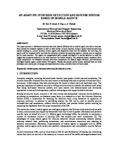
6.1 Performance for optimal m (m-estimate) For the m-estimate parameters, the value of m (equivalent sample size) was varied from 10-300 to 1. As Figure 1 shows, the results for small m (10-44) gave the best results for most data sets. 100%

Accuracy

95% 90%

lpr MIT lpr UNM

85%

sendmail UNM sendmail CERT

80% 75% 1.E-50 1.E-40 1.E-30 1.E-20 1.E-10 1.E+00 equivalent sample size (m) Figure 1. Accuracy

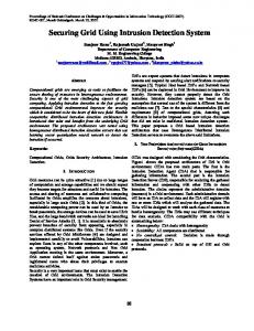
Figure 2 shows the performance for UNM synthetic sendmail dataset varying m. The accuracy achieved was 97.84%, detection rate was 92%, FPR was 1.73% for m=10-44. Furthermore, we profiled our classification using

standard gprof and found out the following time performance: the 10-fold training on lpr MIT dataset took overall 0.26 seconds (including I/O). These results we obtained on a top of the shelf 2.30GHz dual core processor with 4GB physical main memory running a 32-bit operating system. Table 3 shows sample relative errors on posterior probability calculations for both very long and short sequences (183,018 and 7 respectively). These errors have been taken into consideration while determining 78

classification - the grey zone. Let P0 and P1 be the posterior class probabilities given a sequence. The intervals [P0 * (1 - relative error), P0 * (1 + relative error)] and [P1 * (1 - relative error), P1 * (1 + relative error)] are used to classify the sequences. 100% 90% 80% 70% 60% 50%

Accuracy

40%

Detection rate

30%

FPR

20% 10% 0% 1.E-50

1.E-40

1.E-30

1.E-20

1.E-10

1.E+00

Equivalent sample size (m) Figure 2. Performance for UNM synthetic sendmail dataset Table 3. Sample relative errors obtained for synthetic sendmail posterior probabilities (m = 10-50) Actual Sequence Class length 0 183,018 0 3,255 0 7

Posterior probability of class 0 M E Relative error 1.51e-3068 -10 1.98e-14 8.39e-1106 0 3.53e-16 0.01109 0 7.59e-19

Posterior probability of class 1 Predicted M E Relative error class 1.55e-1541 -13 1.98e-14 0 1.49e-1296 0 3.53e-16 0 0.00049 0 7.59e-19 0

We compared our classification results to other popular machine learning techniques. Kang (2005) provides the results of some of those used for misuse-detection. We need to mention that their performance is affected by the bag of system call representation. Table 4 shows the results of our classifier (SC2.2), along with the results on the same four data sets for naïve Bayes multinomial (NBm), the decision tree C4.5, RIPPER (Repeated Incremental Pruning to Produce Error Reduction), support vector machine (SVM), and logistic regression (LR). Table 4. Results on UNM data sets (in percent) Program

SC2.2

NBm

C4.5

RIPPER

SVM

LR

synthetic sendmail Accuracy

97.84

20.21

94.87

94.33

95.68

95.41

Detection rate

92.00

92.00

40.00

48.00

40.00

64.00

84.97

1.15

2.31

0.28

2.31

FPR

1.73

synthetic sendmail CERT Accuracy

96.95

24.39

96.64

95.42

96.03

96.03

Detection rate

91.18

100.00

85.29

82.35

64.70

82.35

2.38

84.35

2.04

3.06

0.34

2.38

FPR

live lpr Accuracy

98.97

83.43

99.91

99.91

100.00

99.91

Detection rate

99.80

100.00

99.80

99.80

100.00

100.00

1.71

30.03

0.00

0.00

0.00

0.16

Accuracy

99.70

54.52

99.89

99.86

99.83

99.97

Detection rate

99.80

100.00

99.90

99.80

99.80

99.90

0.33

62.31

0.11

0.11

0.14

0.00

FPR

live lpr MIT

FPR

79

While the accuracy of our classifier remains comparable or slightly better than that of C4.5, RIPPER, SVM and LR, our detection rate is better than most of them in some data sets, and its accuracy is much better than that of NBm. Moreover, our results take into account the relative error rate while comparing class posterior probabilities. A maximum bound of this error rate was computed based on the relative error of floating-point operations (Kahan, 1997). The difference between posterior probabilities was significant when making the classification decision of test sequences, which gives an accepted level of confidence.

7. CONCLUSION We modeled an arbitrarily long sequence of system calls as a Markov chain. We have implemented a naïve Bayes classifier, where the class-conditional probabilities of a sequence of system calls is computed using a Markov chain model. On one hand, we addressed the issue of zero transitional probabilities that cancel the effect of all the other transitional probabilities. For this purpose, we used the technique of m-estimate of conditional probabilities, finding the value for the equivalent sample size m that yields an optimal compromise between accuracy and detection rate. On the other hand, we addressed the challenge of vanishing probabilities due to multiplying a very large number of probabilities (some sequences contain a few hundred thousand system calls). For this, we used a ―test, backtrack, scale and re-multiply‖ technique, scaling up the conditional probabilities of sequences when they become too small, less than the lowest normal real numbers that can be represented as floating-point numbers. We implemented our technique and benchmarked it against leading classification techniques and found that it yields better compromise on detection rate to accuracy. Furthermore, our classification results take into account the relative error of floating-point operations, which gives the level of confidence in the intrusion detection by leveraging relative error calculations. We intend to use the ROC curve for the identification of an optimal classification model taking into accounts both false positives and true positives. We also intend to extend the work to handle system call parameters.

REFERENCES Chandola, V. et al, 2012. Anomaly detection for discrete sequences: A survey. In IEEE Transactions on Knowledge and Data Engineering. Vol. 24, no. 5, pp. 823-839. Chebrolu, S. et al, 2005. Feature deduction and ensemble design of intrusion detection systems. In Computers and Security. Vol. 24, No. 4, pp. 295–307. Demay, J.-C. et al, 2011. Detecting illegal system calls using a data-oriented detection model. In 26th IFIP International Conference in Security and Privacy for Academia and Industry. Lucerne, Switzerland. Du, W., n.d. Cross-site scripting (XSS) attack lab. Syracuse University, [Online], Available: http://www.cis.syr.edu/~wedu/seed/Labs/Attacks_XSS/XSS.pdf [14 Apr 2013] El Graini, T. et al, 2012. Host intrusion detection for long stealthy system call sequences. IEEE Colloqium on Information Science and Technology. Fez, Morocco. pp.96 – 100. Eskin, E. et al, 2001. Modeling system calls for intrusion detection with dynamic window sizes. Proceedings of DARPA Information Survivability Conference and Exposition II. Anaheim, CA, Vol. 1, pp. 165–175. Farid, D. et al, 2011. Adaptive intrusion detection based on Boosting and Naïve Bayesian classifier. In International Journal of Computer Applications. Vol. 24, No. 3, pp. 12–19. Feng, H. H. et al, 2003. Anomaly detection using call stack information. Proceedings of the IEEE Symposium on Security and Privacy. pp. 62–75. Forrest, S. et al, 1996. A sense of self for Unix processes. IEEE Symposium on Research in Security and Privacy. Oakland, CA, USA, pp. 120–128. Forrest, S., n.d. Computer immune systems – Data sets. University of New Mexico, [Online], Available: http://www.cs.unm.edu/~immsec/systemcalls.htm [14 Apr 2013] Hoang, X.D. and Hu, J., 2004. An efficient hidden Markov model training scheme for anomaly intrusion detection of server applications based on system calls. In IEEE International Conf. Net.. Singapore, Vol. 2, pp. 470–474. Hoang, X. D. et al, 2009. A program-based anomaly intrusion detection scheme using multiple detection engines and fuzzy inference. In Journal of Network and Computer Applications. Vol. 32, No. 6, pp. 1219–1228. Hu, J. et al, 2009. A simple and efficient hidden Markov model scheme for host-based anomaly intrusion detection. In IEEE Network. Vol. 23, No. 1, pp. 42–47. IEEE, 2008. IEEE Standard for floating-point arithmetic. In IEEE Std 754-2008, pp. 1-58. Kahan, W., 1997. Lecture notes on the status of IEEE Standard 754 for binary floating-point arithmetic. Kang, D. et al, 2005. Learning classifiers for misuse and anomaly detection using a bag of system calls representation. Proceedings of the IEEE Workshop on Information Assurance and Security. West Point, NY, USA. pp. 118–125.

80

Krogh, A., 1998. An introduction to hidden Markov models for biological sequences. In Computational Methods in Molecular Biology. Edited by S. L. Salzberg, D. B. Searls and S. Kasif, Elsevier, pp. 45–63. Nadiammai, G. V. et al, 2011. A comprehensive analysis and study in intrusion detection system using data mining techniques. In International Journal of Computer Applications. Vol. 35, No. 8, pp. 51–56. Nidhra, S. and Dondeti, J., 2012. Black box and white box testing techniques – A literature review. In International Journal of Embedded Systems and Applications. Vol. 2, No. 2. Patcha, A. and Park,.J., 2007. An overview of anomaly detection techniques: Existing solutions and latest technological trends. In Computer Networks, Vol. 51, No. 12, pp. 3448–3470. Rabiner, L. R., 1989. A tutorial on hidden Markov model and selected applications in speech recognition. In Proceedings of IEEE. Vol. 77, No. 2. Rao, K. H. et al, 2011. Implementation of anomaly detection technique using machine learning algorithms. In International Journal of Computer Science and Telecommunications. Vol. 2, No. 3, pp. 25–31. Sebek, 2003. Sebek – a kernel based data capture tool. The Honeynet Project. [Online], Available: http://old.honeynet.org/papers/sebek.pdf [14 Apr 2013] Syed, Z. et al, 2009. Learning approximate sequential patterns for classification. In Journal of Machine Learning Research. 10, pp. 1913–1936. Tan, P. et al, 2006. Introduction to data mining. Addison Wesley. Thinh, T. N. et al, 2012. A fpga-based deep packet inspection engine for network intrusion detection system. In International Conference on Electrical Engineering/Electronics, Computer, Telecommunications and Information Technology (ECTICON). pp. 1–4. Wagner, D. and Dean, D., 2001. Intrusion detection via static analysis. Proceedings of the IEEE Symposium on Security and Privacy. Oakland, CA., pp. 156–168. Wang, P. et al, 2010. Survey on HMM based anomaly intrusion detection using system calls. In the 5th International Conference on Computer Science & Education. Hefei, China. Warrender, C. et al, 1999. Detecting intrusions using system calls: Alternative data models. Proceedings of the IEEE Symposium on Security and Privacy. pp. 133–145.

81