not done by the sequential algorithm is termed as the total overhead and is ..... Now consider only the second term of the overhead function and repeat the ...
Isoe�ciency Function: A Scalability Metric for Parallel Algorithms and Architectures Ananth Grama, Anshul Gupta and Vipin Kumar Department of Computer Science, University of Minnesota Minneapolis, MN 55455 This paper provides a tutorial introduction to a performance evaluation metric called the isoe�ciency function. Traditional methods for evaluating serial algorithms are inadequate for
analyzing the performance of parallel algorithm-architecture combinations. Isoe�ciency function has proven useful for evaluating the performance of a wide variety of such combinations. On a sequential computer, the fastest algorithm for solving a given problem is the best algorithm. However, the performance of a parallel algorithm for a speci c problem instance on a given number of processors provides only limited information. The time taken by a parallel algorithm to solve a problem instance depends on the problem size, the number of processors used to solve the problem, and machine characteristics such as: processor speed, speed of communication channels, type of interconnection network, and routing techniques. An algorithm that yields good performance for a selected problem on a xed number of processors on a given machine may perform poorly if any of these parameters are changed. Hence, the evaluation of a parallel algorithm on a parallel computer requires a more comprehensive analysis, and the study of scalability aids us in this analysis. The scalability of a parallel system is a measure of its capacity to deliver linearly increasing speedup with respect to the number of processors used. It re ects the capacity of the parallel system to e�ectively utilize an increasing amount of processing resources. Scalability analysis of an architecture-algorithm combination helps us in answering the following questions: How does increasing the number of processors a�ect the performance of an algorithm? How does changing the problem size a�ect performance? How does changing the computation speed of the processors, or the communication speed of the interconnection network a�ect the performance of a parallel computer for a given algorithm? What is the best algorithm and architecture for solving a problem as the problem size and number of processors change? A number of performance evaluation metrics have been developed to study the scalability of parallel algorithms and architectures [3, 4, 10, 11, 12]. Kumar and Gupta [7] provide a comprehensive survey of di�erent methods of scalability analysis. The isoe�ciency function is one such metric. It relates the size of the problem being solved to the number of processors required to maintain the e�ciency at a xed value. An important feature of the isoe�ciency function is that it succinctly captures the e�ects of characteristics of the parallel algorithm as well as the parallel architecture on which it is implemented, in a single expression. The isoe�ciency function enables us to determine the degree of scalability of a parallel system with respect to the number of processors, the speed of processors, and the communication bandwidth of the interconnection network. Thus 1
we can compare various combinations of parallel algorithms and architectures for a range of problem sizes and number of processors. Hence, using isoe�ciency, we can determine the best parallel algorithm-architecture combination for a problem under a variety of situations without having to explicitly analyze all possible combinations under all possible conditions. The following sections present a discussion of the terminology necessary to use this metric followed by a number of useful examples of isoe�ciency analysis.
1 De nitions and Assumptions In this section, we introduce the terminology used in the rest of the paper. Since a parallel algorithm cannot be evaluated in isolation from the architecture it is implemented on, we de ne a parallel system as the combination of a parallel algorithm and a parallel architecture. Together, a parallel architecture and the parallel algorithm running on it constitute a parallel system. The time taken by an algorithm to execute on a single processor is called the sequential execution time and is denoted by T1. The execution time of the corresponding parallel algorithm on p identical processors is called the parallel execution time and is denoted by TP . A parallel algorithm incurs several overheads during execution. These include overheads due to idling, communication, and contention over shared data structures. The sum total of time spent by all processors doing work which is not done by the sequential algorithm is termed as the total overhead and is denoted by To. In general, To is a function of problem size and the number of processors. Since the sum total of time spent by all processors is pTP , and the total overhead is To, we can see that
pTP = T1 + To or
TP = T1 +p To
(1)
The speedup (S ) obtained from a parallel system is de ned as the ratio of the sequential execution time to the parallel execution time. Therefore,
S = TT1 = T pT+1T P 1 o
The e�ciency (E ) of a parallel system is de ned as the ratio of the speedup obtained to the number of processors used. Therefore,
E = Sp
= T T+1 T 1 o 1 = 1 + TTo
(2)
1
For certain parallel architecture-algorithm combinations, To can be negative. This implies that the speedup obtained from p processors may exceed p. This phenomenon is called superlinear speedup. An example of a parallel system capable of exhibiting such behavior is one in which 2
memory is hierarchical and the access time increases (in discrete steps) with the memory used by the program. In this case, the e�ective computation speed of a large program may be slower on a serial processor than on a parallel computer employing similar processors. This is because a sequential algorithm using M bytes of memory will use only M=p bytes on each processor of a p-processor parallel computer. In this case, cache and virtual memory e�ects may reduce the e�ective computation rate of a serial processor. In order to simplify presentation, we assume that To is non-negative in the rest of the paper. During the course of analyzing parallel systems, we frequently encounter the notion of the size of the problem being solved. So far we have used this term informally without providing a rigorous de nition. One way of expressing the problem size is to represent it by a parameter of the input size. For example, for any matrix problem involving n � n matrices the problem size could be denoted by n. A drawback of this de nition is that the interpretation of problem size changes from one problem to another. For example, doubling the input size results in an 8-fold increase in the serial execution time for matrix multiplication and a 4-fold increase for matrix addition. A better de nition of the size or the magnitude of the problem would be such that irrespective of the problem, doubling the problem size always means performing twice the amount of computation. Therefore, we choose to express problem size in terms of the total number of basic operations inherent in the problem. According to this notion, the problem size for n � n matrix multiplication is �(n3 ), while that for the addition of two n � n matrices is �(n2 ). In order to keep the problem size unique for a given problem, we de ne it as the number of operations the best sequential algorithm executes in order to solve the problem on a single processor. For some problems, the best algorithm is not known; for others, the asymptotically best algorithm may have worse performance than other algorithms for problem instances of interest. In these cases, we can use the number of operations in the serial algorithm that is considered best for such problem instances. For example, for matrix multiplication, the simple �(n3 ) algorithm is often the algorithm of choice, even though Strassen's algorithm has a better asymptotic complexity. The problem size is a function of the size of the input. We will use the symbol W to denote problem size. If the cost of executing each operation is tc , then T1 = Wtc . We illustrate these terms using a simple example.
� Example 1: Adding n numbers on a p-processor hypercube
1
Consider the problem of adding n numbers. For this problem the number of operations, and hence the problem size W is equal to n. If we assume that each addition takes tc time, then T1 is equal to ntc. 1 Now consider a parallel algorithm for adding n numbers using a p-processor hypercube. This algorithm is shown in Figure 1 for n = 16 and p = 4. Each processors is allocated n=p numbers. In the rst step of this algorithm, each processor locally adds its n=p numbers in �(n=p) time. The problem is now reduced to adding the p partial sums on p processors. These can be done by propagating and adding the partial sums as shown in Figure 1. A single step consists of one addition and one nearest neighbor communication of a single word, each of which is a constant time operation. For the sake of simplicity, let us assume that it takes one unit of time to add two numbers and also to communicate a number between two processors. Therefore, n=p time is spent in adding the n=p local numbers at each processor. After the local addition, the p partial sums are added in log p steps, each step consisting In reality the number of basic operations, W , is n ? 1 and the sequential execution time T is given by (n ? 1)tc .
For large values of n, W and T can be approximated by n and ntc respectively. 1
3
1
3
7
11
15
2
6
10
14
1
5
9
13
0
4
8
12
Σ0
3
Σ4
7
Σ8
Σ 12
0
1
2
3
0
1
2
3
2
3
(a) 7
0
15
Σ8 1
15
(b) 15
Σ0
11
2
Σ0 3
0
1
(c)
(d)
Figure 1: Computing the sum of 16 numbers on a 4-processor hypercube. of one addition and one communication. Thus, the total parallel execution time Tp is n=p + 2 log p. The same task can be accomplished sequentially in n time units. Thus, out of the n=p + 2 log p time units that each processor spends in parallel execution, n=p time is spent in performing useful work. The remaining 2 log p units of time per processor contribute to a total overhead of To = 2p log p
(3)
The speedup S and e�ciency E for this algorithm are given by n
S=
T1 = TP
E=
S n = p n + 2p log p
n p
+ 2 log p
(4) (5)
In the next section we formalize the notion of scalability of a parallel system.
2 Scalability of Parallel Systems The number of processors used is an upper bound on the speedup achievable by a parallel system and the speedup for a single processor is one. If more than one processor is used, the speedup obtained is usually less than the number of processors. Let us further investigate how the speedup changes with the number of processors. Consider the problem of adding n numbers on a p-processor hypercube discussed in Example 1. Equations 4 and 5 can be used to calculate the speedup and e�ciency for any given pair of n and p. Figure 2 plots speedup against number of processors for a few di�erent values of n up to 32 processors. Table 1 shows the e�ciencies corresponding to the values of n and p used in Figure 2. Figure 2 and Table 1 illustrate two things. First, for a given problem instance, the speedup does not increase linearly as the number of processors is increased. The speedup curve tends to saturate. In other words, the e�ciency drops with increasing number of processors. This phenomenon is true for all parallel systems, and is often referred to as Amdahl's law. Second, a larger instance of the same problem yields a higher speedup (e�ciency) for the same number of processors. 4
35
Linear 30 25
S
20
n = 512
15
n = 320 n = 192
10
n = 64
5 0 0
5
10
15
20
25
30
35
40
p
Figure 2: Speedup vs. number of processors for adding a list of numbers on a hypercube.
p! n# 64 192 320 512
1 1.0 1.0 1.0 1.0
4
8
16
32
.80 .57 .33 .17 .92 .80 .60 .38 .95 .87 .71 .50 .97 .91 .80 .62
Table 1: E�ciency as a function of n and p for adding n numbers on p-p rocessor hypercubes. Given that increasing the number of processors reduces e�ciency and increasing the size of the computation increases e�ciency, it should be possible to keep the e�ciency constant by increasing both the size of the problem and the number of processors simultaneously. For instance, in Table 1, the e�ciency of adding 64 numbers on a hypercube with four processors is 0.80. If the number of processors is increased to eight and the size of the problem is scaled up to add 192 numbers, the e�ciency remains 0.80. Further increasing p to 16 and n to 512 also results in the same e�ciency. This behavior is exhibited by a large class of parallel systems. For these systems, the e�ciency of parallel execution can be maintained at a constant value by simultaneously increasing the number of processors and the size of the problem being solved. We call such systems scalable parallel systems.
2.1 The Isoe�ciency Metric We have de ned a scalable parallel system as one in which e�ciency can be kept constant as the number of processors is increased, provided that the problem size is also increased. A natural question is, \at what rate should the problem size be increased with respect to the number of 5
processors to keep the e�ciency xed?". For di�erent parallel systems, the size of the problem to be solved has to increase at di�erent rates in order to maintain a xed e�ciency as the number of processors is increased. This rate determines the degree of scalability of the parallel system. In this subsection we introduce a metric for quantitatively determining the degree of scalability of a parallel system. Consider the e�ciency of a parallel algorithm de ned by Equation 2. Substituting T1 = tc W into this equation, we get: (6) E = 1 To 1 + tc W In Equation 6, if the problem size W is kept constant and p is increased, then the e�ciency decreases because the total overhead To increases with p. If W is increased while keeping the number of processors constant, then, for scalable parallel systems, the e�ciency increases. This is because for a given p, To grows slower than �(W ). For these parallel systems, the e�ciency can be maintained at a desired value (between 0 and 1) by increasing p, provided W is also increased. For di�erent parallel systems, W has to be increased at di�erent rates with respect to p in order to maintain a xed e�ciency. For example, in some cases, W might need to grow as an exponential function of p to keep the e�ciency from dropping as p is increased. Such parallel systems are considered poorly scalable. On parallel systems with these characteristics, it is di�cult to obtain good speedups for a large number of processors, unless the size of the problem being solved is enormously large. Conversely, if W needs to grow only linearly with respect to p, then the parallel system is considered highly scalable. This is because it delivers speedups increasing linearly with respect to the number of processors for problem sizes increasing at reasonable rates. For scalable parallel systems, the e�ciency can be maintained at a desired value (between 0 and 1) if the ratio To=W in the expression for e�ciency is maintained at a constant value. To maintain a certain e�ciency E (0 < E < 1), we manipulate Equation 6 to get: To = t ( 1 ? E )
W c E W = t1 ( 1 ?E E )To c
Let K = E=(tc (1 ? E )) be a constant depending on the e�ciency. The equation above can be rewritten as follows:
W = KTo
(7) From Equation 7 the problem size W can usually be obtained as a function of p by algebraic manipulations. This function dictates the rate of growth of W required to keep the e�ciency xed as p is increased. We call this function the isoe�ciency function of the parallel system. The isoe�ciency function of a parallel system determines the ease with which it can achieve speedups increasing in proportion to the number of processors. A small isoe�ciency function implies that small increments in the problem size are su�cient for e�cient utilization of an increasing number of processing elements, and hence the parallel system is highly scalable. Conversely, a large isoe�ciency function indicates a poorly scalable parallel system. The isoe�ciency function does not exist for unscalable parallel systems because in such systems, the e�ciency cannot be kept at constant value as p increases, no matter how fast the problem size is increased. 6
� Example 2:
The expression for the overhead function of the problem of adding n numbers on a p-processor hypercube is given in Equation 3. Substituting the value of To in Equation 7, we get W = 2Kp log p
(8)
Thus the asymptotic isoe�ciency function for this parallel system is �(p log p). This means that if the number of processors is increased from p to p0 , the problem size (in this case, n) will have to be increased by a factor of p0 log p0 =(p log p) to get the same e�ciency as on p processors. In other words, increasing the number of processors by a factor of p0 =p requires n to be increased by a factor of p0 log p0 =(p log p), in order to increase the speedup by a factor of p0 =p.
In the simple example of adding n numbers, the communication overhead is a function of only p. In general, it can depend on both the problem size and the number of processors. A typical
overhead function may have several di�erent terms of di�erent orders of magnitude with respect to p and W . When there are multiple terms of di�erent orders of magnitude in the overhead function, it may be impossible or cumbersome to obtain the isoe�ciency function as a closed form function of p. For instance, consider a hypothetical parallel system, for which To = p3=2 + p3=4W 3=4. In this case Equation 7 will be W = Kp3=2 + Kp3=4W 3=4. It is di�cult to solve for W in terms of p. Recall that the condition for constant e�ciency is that the ratio of To and W should remain xed. As p and W increase in a parallel system, the e�ciency is guaranteed not to drop if none of the terms of To grow faster than W . Therefore, if To has multiple terms, we balance W against each individual term of To to compute the respective isoe�ciency function. The component of To that causes the problem size to grow at the fastest rate with respect to p determines the overall asymptotic isoe�ciency function of the computation.
� Example: 3 Consider a hypothetical parallel algorithm-architecture combination for which To = p3=2 + p3=4W 3=4. If we ignore the second term of To and use only the rst term in Equation 7, we get W = Kp3=2
(9)
Now consider only the second term of the overhead function and repeat the above analysis. Equation 7 now takes the form W = Kp3=4W 3=4 W 1=4 = Kp3=4 W = K 4 p3
(10)
In order to ensure that the e�ciency does not decrease as the number of processors increase, the rst and the second term of the overhead function require the problem size to grow as �(p3=2) and �(p3 ), respectively. The asymptotically higher of the two rates should be regarded as the overall asymptotic isoe�ciency function. Thus, the isoe�ciency function is �(p3 ) for this parallel system. This is because if the problem size W grows as �(p3 ), then To would remain of the same order as W .
7
By performing isoe�ciency analysis, we can test the performance of a parallel program on a few processors, and then predict its performance on a larger number of processors. However, the utility of the isoe�ciency analysis is not limited to predicting the impact on performance of an increasing number of processors. As we shall see in later sections, it can also be used to study the behavior of a parallel system with respect to changes in other hardware related parameters, such as the speed of the processors and the data communication channels.
2.2 Cost-Optimality and Isoe�ciency Function
A parallel system is cost-optimal if the product of the number of processors and the parallel execution time is proportional to the execution time of the best known serial algorithm on a single processor. In other words, a parallel system is cost-optimal if and only if
pTP / W Substituting TP from the right hand side of Equation 1, we get
T1 + T o / W Since T1 = Wtc , we have
Wtc + To / W W / To
(11) Equation 11 suggests that a parallel system is cost-optimal if its overhead function and the problem size are of the same order of magnitude. This is exactly the condition required to maintain a xed e�ciency while increasing the number of processors in the parallel system (Equation 7). It follows then that conforming to the isoe�ciency relation between the problem size and the number of processors is a way to retain the cost-optimality of a parallel system as it is scaled up.
2.3 A Lower Bound on Isoe�ciency Function We discussed earlier that a smaller isoe�ciency function indicates better scalability. A natural question to ask then is: how small an isoe�ciency function can be and what is an ideally scalable parallel system? If a problem consists of W basic operations, then no more than W processors can be used to solve the problem in a cost-optimal fashion. If the problem size grows at a rate slower than �(p) as the number of processors increases, then eventually the number of processors will exceed W , and, even in an ideal parallel system with no communication or other overheads, the e�ciency will drop because the processors exceeding W will have no work to do. Thus asymptotically, the problem size has to increase at least as fast as �(p) to maintain a constant e�ciency and hence (p) is the asymptotic lower bound on the isoe�ciency function. It also follows that the isoe�ciency function of an ideally scalable parallel system is �(p).
2.4 Degree of Concurrency and Isoe�ciency Function The lower bound of (p) is imposed on the isoe�ciency function of a parallel system by the number of operations that can be performed concurrently. We de ne the maximum number of tasks that can 8
be executed simultaneously at any given time in a parallel algorithm as its degree of concurrency. The degree of concurrency is a measure of the number of operations that an algorithm can perform in parallel in a problem of size W and is independent of the parallel architecture. If C (W ) is the degree of concurrency of a parallel algorithm, then given a problem of size W , at most C (W ) processors can be employed e�ectively. For example, using Gaussian elimination to solve a system of n equations with n variables, the total amount of computation is �(n3 ). However, the n variables have to be eliminated one after the other, and eliminating a particular variable involves �(n2 ) computations. Thus, at most O(n2) processors can be kept busy at any given time. Now if W = �(n3) for this problem, then the degree of concurrency C (W ) is �(W 2=3). Since, if given a problem of size W , at most �(W 2=3 ) processors can be used, then given p processors, the size of the problem should be at least (p3=2) in order to use all the processors. Thus, the isoe�ciency function of this computation due to concurrency is �(p3=2). The isoe�ciency function due to concurrency is optimal (i:e:, �(p)) only if the degree of concurrency of the parallel algorithm is �(W ). If the degree of concurrency of an algorithm is less than �(W ), then the isoe�ciency function due to concurrency can be worse (greater) than �(p). In such cases, the overall isoe�ciency function of a parallel system is given by the maximum of the isoe�ciency functions due to concurrency, communication, and other overheads.
3 Illustrations of Isoe�ciency Analysis In this section, we illustrate the utility of isoe�ciency analysis using di�erent examples. Often we are faced with a need for comparing the performance of two parallel algorithms for a large number of processors. The asymptotic isoe�ciency function provides us with such a tool. The algorithm with the smaller asymptotic isoe�ciency function yields better performance as the number of processors becomes large. We illustrate this in Subsection 3.1 using the example of two parallel algorithms for computing the matrix-vector product. For certain parallel systems, changing speed of processors and communication channels impacts scalability moderately. However, for some other parallel systems, this impact is signi cant. This e�ect of machine speci c parameters on the scalability is illustrated in Subsection 3.2 in the context of a parallel algorithm for computing Fast Fourier Transforms. Some parallel algorithms have low overhead due to communication, idling and contention, but o�er limited concurrency. For many of these algorithms, concurrency plays a critical role in determining the overall isoe�ciency. We illustrate this using Dijkstra's all pairs shortest path algorithm in Subsection 3.3. There are other algorithms which have a low overhead due to communication and idling, and o�er a high degree of concurrency, but su�er from contention over shared data structures. For many of these algorithms, it is di�cult to analytically model the overheads due to contention. In Subsection 3.4, we demonstrate in the context of the dynamic load balancing problem how the isoe�ciency function can be used to determine the scalability of such algorithms.
3.1 Comparing two parallel algorithms The asymptotic values of the isoe�ciency function can be used to compare the performance of various algorithms as the number of processors becomes large. We illustrate this using the example of two parallel algorithms for computing a matrix-vector product on a hypercube connected 9
computer.
� Example 4: Stripe Based Matrix-Vector Product on a Hypercube Consider the problem of multiplying an n � n matrix with an n � 1 vector. The number of basic operations needed for this matrix-vector product, and the problem size W is equal to n2. If the time taken by a single addition and multiplication operation is tc , then the sequential execution time of this algorithm is n2tc ; i.e., T1 = n2 tc [5]. Matrix A
Vector x
Processors
P0
0
P0
P1
1
P1
. .
n
Pp-1
p-1
(a) Initial partitioning of the matrix and the starting vector x
1
. .
n/p
Pp-1
0
p-1
(b) Distribution of the full vector among all the processors by all-to-all broadcast Matrix A
Vector y
P0
0
1
p-1
P0
0
P1
0
1
p-1
P1
1
0
1
p-1
0
1
p-1
. .
0
1
p-1
Pp-1
. . Pp-1
p-1
(d) Final distribution of the matrix and the result vector y
(c) Entire vector distributed to each processor after the broadcast
Figure 3: Multiplication of an n � n matrix with an n � 1 vector using row-wise striped data partitioning. Figure 3 illustrates a parallel formulation of this algorithm based on striped partitioning of the matrix and the vector. Each processor is assigned n=p rows of the matrix and n=p elements of the vector. Since the matrix-vector multiplication requires the vector to be multiplied with each row of the matrix, every processor needs the entire vector. In order to accomplish this, in the rst step, each processor broadcasts its n=p elements of the vector to every other processor. This operation is also referred to as an all-to-all broadcast. After this step, each processor has the vector available locally and n=p rows of the matrix. Using these, it computes the dot products locally, and at the end of this step, each processor has n=p elements of the resulting vector. Let us now analyze the performance of this parallel formulation for a hypercube connected computer. The rst step of the algorithm involving the all-to-all broadcast of packets of size n=p among p
10
processors can be performed in ts log p + tw n(p ? 1)=p time [5]. Here, ts is the startup time of the communication network and tw is the per-word transfer time. For large values of p this can be approximated to ts log p + tw n. Assuming that an addition and a multiplication takes tc units of time, each processor spends tc n2=p units of time in multiplying its n=p rows with the vector. Thus, the parallel execution time of this procedure is given by: TP = tc
n2 + ts log p + tw n p
(12)
The corresponding speedup S and e�ciency E are given by: S= E=
p
1+
p(ts log p+tw n) tc n2
1+
tsp log p+tw np tc n2
1
(13) (14)
Now we derive an expression for the isoe�ciency function for this parallel formulation. Using the relation To = pTP ? T1 , we get the following expression for the overhead function of the striped matrix-vector multiplication on the hypercube: To = tsp log p + tw np
(15)
We can determine the isoe�ciency function from the equation W = KTo (Equation 7). Let us rewrite this relation for our parallel formulation of matrix-vector multiplication, rst with only the ts term of To . W = Kts p log p
(16)
Equation 16 gives the isoe�ciency term with respect to the message startup time. Similarly, the tw term of the overhead function can be balanced against the problem size W as follows: n2 = Ktw np n = Ktw p W = n2 = K 2 t2w p2
(17)
From Equations 16 and 17 it can be inferred that the overall asymptotic rate at which the problem size needs to increase with the number of processors in order to maintain a xed e�ciency is �(p2 ).
� Example 5: Checkerboard Based Matrix-Vector Product on a Hypercube Consider an alternate partitioning of the matrix and the vector for computing the matrix-vector product. Instead of partitioning the matrix into stripes, we now divide it into p squares, each of dimensions (n=pp) � (n=pp). This partitioning is referred to as checkerboard partitioning [5]. The parallel matrix-vector multiplication algorithm based on this partitioning is illustrated in Figure 4. The vector itself is distributed along the last column of the mesh. In the rst step of the algorithm, the vectorpis aligned along the diagonal processors. For this, all processors of the last column send their n= p elements of the vector to pthe diagonal processor of their respective rows. Then a column-wise one-to-all broadcast of these n= p elements is performed.
11
P0 P1 Ppp P pp 2
. .
n=pp
Vector x
Matrix A
Ppp
-1
pnp
n
. . Pp
-1
(a) Initial data distribution and communication steps to align the vector along the diagonal
(b) One-to-all broadcast of portions of the vector along processor columns Vector y
Matrix A
P0 P1 Ppp P pp 2
. .
Ppp
-1
. . Pp
-1
(c) Single-node accumulation of partial results
(d) Final distribution of the result vector
Figure 4: Matrix-vector multiplication using checkerboard partitioning. After this communication step, the vector is aligned alongpthe rows of the matrix. Each processor performs n2 =p multiplications and locally adds up the n= p sets of products. As shown in Figure 4(c), each processor now has n=pp partial sums which need to be accumulated along each row to obtain the resultant vector. Hence, the last step of the algorithm is a single node accumulation of these n=pp values in each row, with the last processor of the row as the destination. The operation of this algorithm is illustrated in Figure 4. We now analyze the performance of this algorithm on a hypercube connected computer with store and forward routing [5]. The rst step of sending a messagepfrom the last processor of a row to the diagonal processor can be performed in at most ts + tw (n= p) log pp. The second communication step distributes copies of the vector among the rows of processors and involves one-to-all broadcasts in all the pcolumnspof processors as shown in Figures 4(b) and 4(c). This step can be performed in (ts + tw n= p) log p. If a multiplication and an addition is assumed to take tc units of time, then each processors spends approximately tcn2 =p time performing computation. Now if the resultant vector has to be placed in the last column of processors like the starting vector, then a single node accumulation p of components of size n= p of the vector has to be performed in each row of processors. Ignoring the time required for performing additions during this step, the accumulation can be performed with a communication time of (ts + tw n=pp) log pp. Summing up the time taken by all the steps, the total parallel execution time for this procedure is given by the following equation :
12
TP = t c
n2 n p p + ts + 2ts log p + 3tw p log p p p
This can be approximated by TP = tc
3 n n2 + ts log p + tw p log p p 2 p
(18)
From this equation, the total overhead To is given by: 3 p To = ts p log p + tw n p log p 2 As before, we can equate each term in this overhead function with the problem size W . For the isoe�ciency due to ts , we have W / Kts p log p, where K = 1=(tc(1 ? E )). For isoe�ciency due to tw , equating W with KTo , we have 3 p n2tc = K tw n p log p 2 t p 3 n = K w p log p 2 tc 9 t2 n2 = K 2 w2 p log2 p 4 tc Therefore, the isoe�ciency due to tw is given by �(p log2 p). Since this term asymptotically dominates the �(p log p) term due to ts , the overall isoe�ciency of this formulation is given by �(p log2 p).
From these two examples, we can see that the isoe�ciency function of the stripe based matrixvector product algorithm is �(p2 ), because it is asymptotically higher than the �(p log2 p) isoe�ciency function of the checkerboard based algorithm. This implies that as the number of processors is increased, the stripe based formulation will require much larger problem sizes to yield the same e�ciencies as the checkerboard based formulation.
3.2 Predicting e�ects of machine speci c parameters Isoe�ciency analysis can be used to predict the e�ect of such machine speci c parameters as processor speed and speed of communication channels (startup time, per-word transfer time, etc:). In this section, we illustrate how isoe�ciency analysis is useful in making such predictions.
� Example 6: Fast Fourier Transforms Consider the Cooley-Tukey algorithm for computing an n-point single dimensional unordered radix-2 FFT [2, 5]. Figure 5 illustrates the algorithm graphically. The sequential complexity of this formulation is given by �(n log n). In this section, we will use a parallel formulation of this algorithm based on the binary exchange method for a hypercube based computer. In this parallel formulation, shown in Figure 5, we partition the vectors into blocks of n=p contiguous elements and assign one such block to each processor. Let the hypercube being used be d-dimensional (i:e:, p = 2d ) and let n = 2r . An interesting property of the mapping shown in Figure 5 is that the vector elements residing on di�erent processors are combined during the rst d iterations, while the pairs of elements combined during the
13
m=0
m=1
m=2
m=3
X[0]
Y[0]
X[1]
Y[1]
X[2]
Y[2]
X[3]
Y[3]
X[4]
Y[4]
X[5]
Y[5]
X[6]
Y[6]
X[7]
Y[7]
X[8]
Y[8]
X[9]
Y[9]
X[10]
Y[10]
X[11]
Y[11]
X[12]
Y[12]
X[13]
Y[13]
X[14]
Y[14]
X[15]
Y[15]
P0
P1
P2
P3
Figure 5: A 16-point FFT on four processors. Pi denotes processor number i and m refers to the iteration number. last (r ? d) iterations reside on the same processors. Hence, this parallel FFT algorithm involves interprocessor communication only during d = log p of the log n iterations. Each communication operation involves exchanging n=p words of data. Thus, the time spent in communication during the execution of the entire algorithm is (ts + tw n=p) log p. In each iteration, a processor updates n=p elements of vector R. If a complex multiplication and addition takes time tc , then the parallel execution time of the n-point parallel FFT on a p-processor hypercube is given by: n n TP = tc log n + ts log p + tw log p p p From this equation, we can also see that the total overhead To is given by:
(19)
To = ts p log p + tw n log p
We know that the problem size for an n-point FFT is given by: W = n log n
(20) Following the methodology of Examples 4 and 5, we can determine the isoe�ciency by equating the problem size with the total overhead. For isoe�ciency due to ts, we have W / ts p log p, which
14
corresponds to an isoe�ciency function of �(p log p). The isoe�ciency due to the tw term can also be determined similarly: n log n log n n n log n
= = = =
Ktw n log p Ktw log p tw p K tc Ktw pKtw log p
E tw 1?EE twc log p (21) 1 ? E tc p If the term tw E=(tc (1 ? E )) is less that 1, then the rate of growth of problem size dictated by Equation 21 is less than �(p log p), and hence the overall isoe�ciency function is �(p log p) for this parallel system. On the other hand, if tw E=(tc (1 ? E )) exceeds 1, then Equation 21 determines the overall isoe�ciency function which is now greater than �(p log p). Also, in this case, the asymptotic isoe�ciency function depends on the relative values of E=(1 ? E ), tw and tc . Thus, the FFT algorithm is somewhat unique in that the asymptotic isoe�ciency function is a function of the desired e�ciency and hardware dependent parameters. In fact the e�ciency corresponding to tw E=(tc (1 ? E )) = 1, (i:e:, E=(1 ? E ) = tc =tw , or E = tc =(tc + tw )) acts as a threshold value. For a given hypercube connected computer with xed tc and tw , e�ciencies up to this values can be obtained easily. But e�ciencies much higher than this threshold can be obtained only if the problem size is extremely large. Let us examine the e�ect of the value of tw E=(tc (1 ? E )) on the isoe�ciency function. Consider the computation of an n-point FFT on a p-processor hypercube on which tw = tc . The isoe�ciency function of the parallel FFT on this machine is E=(1 ? E )pE=(1?E ) log p. Now for E=(1 ? E ) � 1 (i.e. E � 0:5) the overall isoe�ciency is �(p log p), but for E > 0:5, the isoe�ciency function is much worse. For instance, if E = 0:9, then E=(1 ? E ) = 9 and hence the isoe�ciency function becomes �(p9 log p). Now consider the computation of an n-point FFT on a p-processor hypercube on which tw = 2tc . The threshold e�ciency is 0.33. The isoe�ciency function for E = 0:33 is �(p log p), for E = 0:5 it is �(p2 log p), and for E = 0:9 it becomes �(p18 log p). t
W=
The above examples show that there is a limit on the e�ciency that can be obtained for reasonable problem sizes, and this limit is determined by the ratio of the CPU speed and the bandwidth of the communication channels of the hypercube. This limit can be raised by increasing the bandwidth of the communication channels. On the other hand, making the CPU's faster without improving the communication bandwidth lowers this threshold. Hence, this parallel formulation of FFT performs poorly on a hypercube whose communication and computation speeds are not balanced. If the hardware is balanced with respect to communication and computation speeds, then the FFT algorithm is fairly scalable on a hypercube with an overall isoe�ciency function of �(p log p), and good e�ciencies can be expected for reasonably large number of processors. This example illustrates how the isoe�ciency function can be used to derive the e�ect of various machine speci c factors. For a more detailed scalability analysis of this and other parallel FFT algorithms, see [2, 5].
3.3 Impact of Concurrency on Scalability We have seen that the maximum concurrency in a parallel algorithm often limits the number of processors that can be e�ectively utilized. Therefore, the problem size has to grow fast enough 15
so that it is possible to use the increased number of processors. For many algorithms limitations imposed by concurrency plays a dominant role in determining overall scalability. We illustrate this in the context of Dijkstra's all pairs shortest path algorithm.
� Example 7: Dijkstra's All Pair's Shortest Path Algorithm Consider the all-pairs shortest path problem for a dense graph with n vertices. The problem involves nding the shortest path between each pair of vertices in the graph. The best known serial algorithm for solving this takes time �(n3 ) time. This problem can also be solved using n instances of the singlesource shortest path problem. The single source shortest path problem determines the shortest path from one vertex to every other vertex in the graph. The sequential complexity of the single-source shortest path problem is �(n2 ). Therefore, by executing one instance of the single-source shortest path algorithm for each of the n vertices, we can solve the all-pairs shortest path problem. A simple parallel formulation of this algorithm can be derived by using n processors with each processor executing a single-source shortest path problem independently. Since each of these computations is independent of the other, the parallel formulation requires absolutely no communication. It may therefore seem that this algorithm is the best possible algorithm. Let us consider the scalability resulting from the concurrency in this parallel algorithm. Since the algorithm can use at most n processors, p = n, and since the problem size W is �(n3 ), W must grow at least as �(p3 ) to be able to use additional processors. This function determines the overall isoe�ciency of the parallel formulations. This isoe�ciency is relatively high and other algorithms with better isoe�ciencies are available.
This example illustrates how isoe�ciency captures the concurrency inherent in a parallel algorithm. An algorithm may appear attractive because of lack or absence of communication, but may indeed perform poorly for higher number of processors because of limited concurrency. See [5, 9] for scalability analysis of a number of other shortest-path algorithms.
3.4 Impact of Contention for Shared Data Structures For some parallel algorithms, it is di�cult to compute the parallel execution time analytically, as the e�ects of certain overheads such as those due to contention are di�cult to model. In such applications, isoe�ciency analysis may still be a useful tool for analyzing the scalability. In this subsection, we present one such parallel algorithm.
� Example 8: Dynamic Load Balancing Consider an application with the following characteristics:
{ The work available at any processor can be partitioned into independent work pieces as long as
it is more than some non-decomposable unit. { It is di�cult to estimate the amount of computation associated with a piece of work. { A reasonable work splitting mechanism is available; i:e:, if work w at one processor is partitioned into two parts w and (1 ? )w, then there exists an arbitrarily small constant �(> 0), such that w > �w and (1 ? )w > �w. The role of � is to set a bound on the load imbalance resulting from work splitting.
16
Instances of applications which conform to these characteristics are found in depth rst search of large unstructured trees used for solving discrete optimization problems [6]. Some parallel algorithms for solving this problem employ the following dynamic load balancing strategy. All work is initially assigned to one processor. An idle processor Pi selects a processor Pa using some selection criterion and sends it a work request. If processor Pa has no work, then it responds with a reject message; else, it partitions its work into two parts and sends one of the pieces to Pi. This process continues until all processors exhaust the available work. Various selection criteria have been proposed in literature [6, 8]. One technique referred to as Global Round Robin (GRR) maintains a global pointer G located at one of the processors. This pointer initially points to the rst processor in the ensemble. Each time an idle processor needs to select Pa , it reads the current value of G, and requests work from PG. Before the next request from an idle processor is processed, the global pointer is incremented by one (modulo p). The global pointer distributes the work requests evenly over the various processors. We can see that the non-deterministic nature of the algorithm makes it impossible to evaluate the exact parallel execution time of such an algorithm. However, it is possible to bound the communication cost of such an algorithm. As shown in [6, 5], an upper bound on the number of communications required for this algorithm is O(p log W ). Each communication takes O(log p) time, and the total overhead resulting from the communication of work is bounded by O(p log p log W ). As before, this term can be equated with the problem size W to yield the isoe�ciency resulting from communication overheads. Therefore, W / O(p log p log W ) Substituting the value of W from the right hand side of the expression back into the right hand side and ignoring the double log terms, we can see that the isoe�ciency of this algorithm due to communication overheads is O(p log2 p). This term however does not specify the overall isoe�ciency of the system because the algorithm has overheads in addition to that for communicating work. In this algorithm a global variable is accessed repeatedly. If many processors try to access it at the same time, then only one will succeed, and others will have to wait due to contention. We analyze the isoe�ciency due to contention as follows: The global variable is accessed O(p log W ) number of times (for read and increment operations) over the entire execution. If processors are e�ciently utilized, then the total time of execution is �(W=p). Assume that while solving some speci c problem instance of size W on p processors, there is no contention. In this case, W=p is much more than the total time over which the shared variable is accessed. Now, as we increase the number of processors, the total time of execution ( i:e:, W=p ) decreases but the number of times the shared variable is accessed increases. There is thus a crossover point beyond which the shared variable access will become a bottleneck and the overall execution time cannot be reduced further. This bottleneck can be eliminated by increasing W at a rate such that the ratio between W=p and O(p log W ) remains the same. Equating W=p and O(p log W ) and simplifying yields an isoe�ciency term of O(p2 log p). Thus, since the isoe�ciency due to contention asymptotically dominates the isoe�ciency due to communication, the overall isoe�ciency is given by O(p2 log p).
In this example, we have seen how it is possible to model overheads due to contention using the isoe�ciency metric. A number of other dynamic load balancing algorithms have been analyzed in [6, 8]. In [6], it is experimentally shown that dynamic load balancing schemes with better isoe�ciency functions outperform those with poorer isoe�ciency functions.
17
4 Summary and Concluding Remarks The isoe�ciency metric is useful in situations in which we are interested in obtaining linearly increasing performance with the number of processors. If the rate of growth of problem size is the same as that speci ed by the isoe�ciency function, then the speedup obtained from the parallel system is linear. In certain cases, it may not be possible or desirable to increase the problem size at the rate speci ed by the isoe�ciency function. If this rate is smaller than the isoe�ciency then the speedup is sublinear. For a given rate of growth of problem size, the speedup curve can be used as a scalability metric. If the problem size is increased linearly with the number of processors, the speedup curve is referred to as scaled speedup [3]. The rate of growth of problem size may also be constrained by the amount of memory in the parallel computer. In this case, the problem size is increased at the fastest rate allowed by the available memory. These metrics have been investigated by Worley [12], Gustafson [3] and Sun and Ni [10]. In many situations, the rate of growth of problem size is dictated by the time available to solve the problem. In these cases, the problem size is increased with number of processors in such a way that the parallel runtime remains constant. The scalability issues for such problems have been explored by Worley [12], Gustafson [3], and Sun and Ni [10]. It is also possible to keep the problem size xed and use the speedup curve as a scalability metric. Performance issues related to xed problem size case have been addressed in [1]. There are certain interesting relationships between isoe�ciency and some of these metrics. It can be shown that if the isoe�ciency function is greater than �(p), then for a scalable parallel system, the problem size cannot be increased inde nitely while maintaining a xed execution time, no matter how many processors are used [1, 7]. In [1], we have shown that for a class of parallel systems, the relationship between the problem size and the number of processors on which the problem executes in minimum time is speci ed by the isoe�ciency function.
Acknowledgements This work was supported by Army Research O�ce grant #28408-MA-SDI to the University of Minnesota and by the Army High Performance Computing Research Center at the University of Minnesota. The authors would also like to thank Daniel Challou for his help in the preparation of this document.
References [1] Anshul Gupta and Vipin Kumar. Performance properties of large scale parallel systems. Journal of Parallel and Distributed Computing (special issue on supercomputer performance), November 1993. Also available as Technical Report 92-32, Department of Computer Science, University of Minnesota, Minneapolis, MN. [2] Anshul Gupta and Vipin Kumar. The scalability of FFT on parallel computers. IEEE Transactions on Parallel and Distributed Systems, 4(8):922{932, August 1993. A detailed version available as Technical Report TR 90-53, Department of Computer Science, University of Minnesota, Minneapolis, MN. 18
[3] John L. Gustafson. Reevaluating Amdahl's law. Communications of the ACM, 31(5):532{533, 1988. [4] John L. Gustafson. The consequences of xed time performance measurement. In Proceedings of the 25th Hawaii International Conference on System Sciences: Volume III, pages 113{124, 1992. [5] Vipin Kumar, Ananth Grama, Anshul Gupta, and George Karypis. Introduction to Parallel Computing: Design and Analysis of Algorithms. Benjamin/Cummings, Redwood City, CA, 1994. [6] Vipin Kumar, Ananth Grama, and V. Nageshwara Rao. Scalable load balancing techniques for parallel computers. Technical Report 91-55, Computer Science Department, University of Minnesota, 1991. To appear in Journal of Distributed and Parallel Computing, 1994. [7] Vipin Kumar and Anshul Gupta. Analyzing scalability of parallel algorithms and architectures. Technical Report TR 91-18, Department of Computer Science Department, University of Minnesota, Minneapolis, MN, 1991. To appear in Journal of Parallel and Distributed Computing, 1994. A shorter version appears in Proceedings of the 1991 International Conference on Supercomputing, pages 396-405, 1991. [8] Vipin Kumar and V. N. Rao. Parallel depth- rst search, part II: Analysis. International Journal of Parallel Programming, 16(6):501{519, 1987. [9] Vipin Kumar and Vineet Singh. Scalability of Parallel Algorithms for the All-Pairs Shortest Path Problem. Journal of Parallel and Distributed Computing, 13(2):124{138, October 1991. A short version appears in the Proceedings of the International Conference on Parallel Processing, 1990. [10] Xian-He Sun and L. M. Ni. Another view of parallel speedup. In Supercomputing '90 Proceedings, pages 324{333, 1990. [11] Xian-He Sun and Diane Thiede Rover. Scalability of parallel algorithm-machine combinations. Technical Report IS-5057, Ames Laboratory, Iowa State University, Ames, IA, 1991. To appear in IEEE Transactions on Parallel and Distributed Systems. [12] Patrick H. Worley. The e�ect of time constraints on scaled speedup. SIAM Journal on Scienti c and Statistical Computing, 11(5):838{858, 1990.
19