J17.1
MODEL- AND APPLICATION-SPECIFIC VALIDATION DATA FOR LES-BASED TRANSPORT AND DIFFUSION MODELS
M-Y. Lee1*, F. Harms2, T. Young1, B. Leitl2, and G. Patnaik3 Berkeley Research Associates, Beltsville MD, 2University of Hamburg, Hamburg, Germany, 3Naval Research Laboratory, Washington DC
1
1.
INTRODUCTION
Numerical simulations of dispersion in an urban environment are complex and require substantial computational effort. Simpler models such as empirical (Gaussian) models, diagnostic models (which use only the mass conservation equation) or Computational Fluid Dynamics (CFD) models with full parameterization of turbulence, i.e., Reynolds-averaged Navier-Stokes (RANS) codes were used in the past for these complex tasks. Simplified models can compute urban dispersion within a reasonable amount of time, but they are unable to capture the inherently unsteady plume dynamics driven by urban geometry. Direct numerical simulations (DNS) are simulations where the Navier-Stokes equations are numerically solved without any turbulence model. These simulations are able to compute transient flow dynamics, but they are prohibitively expensive for most practical flows at moderate-to-high Reynolds numbers, and especially so for urban contaminant transport (CT) studies. Large Eddy Simulation (LES) constitutes an effective intermediate approach between DNS and the RANS methods (Sagaut, 2004). LES is capable of simulating flow features that cannot be handled with RANS such as significant flow unsteadiness and localized vortex shedding, and provides higher accuracy than the industrial methods at lower cost. LES solutions converge to the solutions of the Navier-Stokes equations as resolution is increased, whereas RANS generally do not. Because the larger-scale unsteady features of the flow govern the unsteady plume dynamics in urban geometries, the LES approximation can capture some key features which the RANS methods and the various Gaussian plume methodologies cannot. Nowadays increasing computer power enabled the possibility to use LES models for urban dispersion simulations.
*Corresponding author address: MiYoung Lee, Berkeley Research Associates, 6551 Mid Cities Ave., Beltsville, MD 20705-1434; email:
[email protected]
Establishing the credibility of urban CFD solutions has been one of the stumbling blocks to their widespread use. Code validation using experiments requires well-characterized datasets with information adequate for defining and evaluating unsteady simulations. Unfortunately, current fullscale field studies do not fully provide this information. The number of trials is limited and the data acquired is typically too sparse and/or insufficient to properly characterize the flows. Further, the inherent variability of the experimental results cannot be measured from these data. Validation data for numerical models are not just any experimental data; they must fulfill certain requirements with respect to completeness, spatial and temporal resolution, accuracy, representativeness and documentation of the measured results (Schatzmann, et al., 2002). If these requirements are not met, too many degrees of freedom remain to set-up unique numerical model runs. A wide variety of numerical results can be generated with reasonable assumptions for the input data, with the consequence that a solid conclusion concerning the model quality cannot be reached. To overcome these problems, datasets that match the complexity of specific groups of models are needed. For the validation of Large Eddy Simulation models for urban applications, data are needed that comprise flow and turbulence fields in combination with concentration fields measured with high resolution in space and time within the urban boundary layer. Field trials are essential for validation but do not yet provide complete validation data. In addition, specific data are required that test the particular parameterizations this model type applies. Under certain limiting conditions, such datasets can be generated under carefully controlled conditions in well-equipped boundary layer wind tunnels. The results presented here were obtained as part of a joint research project of the Meteorological Institute of the University of Hamburg and the Naval Research Laboratory. Two of the goals of this study were: 1. to create benchmark quality datasets for the validation of time-resolved urban CFD models such as FAST3D-CT,
2. to create a description for data acquisition and reduction to adequately characterize turbulent inflow and wind variability for urban CT models. 2.
was 3.5 m, corresponding to 1050 m at full-scale. The spires and floor roughness elements can be seen upstream of the test section with the OKC model.
BRIEF OUTLINE OF THE WIND TUNNEL EXPERIMENTS
The aim of the wind tunnel measurements was to create a high quality reference dataset that is adequate to fulfill major model- and applicationspecific validation data requirements for an LESbased, urban flow and dispersion model. Numerous flow and concentration measurements in two extended six-month wind tunnel campaigns were carried out. Oklahoma City was selected because one of the most extensive field campaigns in urban areas, Joint Urban 2003 (JU2003), was conducted there (Doran 2007). The wind tunnel measurements were carried out in the University of Hamburg’s large boundary layer wind tunnel facility 'WOTAN' (Figure 1). The 25 m long wind tunnel provides an 18 m long test section equipped with two turntables and an adjustable ceiling. The cross section of the tunnel measures 4 m in width and 2.75 to 3.25m in height, depending on the position of the adjustable ceiling.
Figure 2. Wind tunnel model of the Central Business District of Oklahoma City.
For dispersion modeling and measurements, at ground level several point emission sources were flush-mounted in the model. The circular release area had a diameter of 7 mm (model scale), corresponding to 2.1 m at full scale. To avoid the formation of a significant vertical jet at higher emission rates, the source area was covered by a top, 3.5 mm (1.05 m full-scale) above ground level. Figure 3 shows two of the sources mounted near the Westin Hotel.
Figure 1. The large boundary layer wind tunnel facility 'WOTAN' of the University of Hamburg.
While free stream wind speeds of more than 20 m/s can be realized in the test section, the typical wind velocities chosen for atmospheric flow and dispersion modeling are in the range of 5 m/s to 15 m/s. The model boundary layer flow is generated by a carefully optimized combination of turbulence generators (~spires) at the inlet of the test section and a floor roughness. Figure 2 shows the wind tunnel model of the Central Business District of Oklahoma City (OKC) mounted in the wind tunnel in the scale of 1:300. The diameter of the detailed wind tunnel model
Figure 3. Two sources mounted next to the Westin Hotel.
The modeled release locations were chosen in accordance with some of the release sites used during the JU2003 field campaign. In order to simulate instantaneous puff releases, a continuous by-pass flow of tracer gas was temporarily switch-
ed to the source by means of a fast solenoid micro-valve. With this setup, the release rate could be kept constant for repetitive releases lasting much less than a second at model scale. The precise repeatability of releases and the consistency of puff modeling were verified by extensive systematic test series prior to the actual model tests. A Fast Flame Ionization Detector mounted to a traverse system measured puff dispersion. Whereas sampling took place near the ground, the instrument was located well above the urban structures to avoid flow disturbances by the instrument (Figure 4).
Figure 4. Fast Flame Ionization Detector within the model of Oklahoma City.
During the first wind tunnel campaign, flow measurements with a high temporal and spatial resolution within the model area were carried out. A 2D Laser Doppler Anemometer system (LDA) provided flow data at sampling rates of several hundred Hertz (up to more than 1 kHz under favorable conditions), resolving even small-scale turbulence in time. More than 2500 individual flow measurements at different locations were done to provide a high spatial resolution within the model area. The second objective of the first wind tunnel campaign was to characterize the inflow conditions upstream of the Oklahoma model as precisely as possible. Therefore, the development of the boundary layer within the approach section of the wind tunnel was measured, documented and analyzed, and the modeled boundary layer at the end of the approach flow section upstream of the model was characterized by corresponding measurements. During the second wind tunnel campaign, the dispersion of puffs in urban environments was analyzed by systematic measurements. A major goal of these measurements was to evaluate the
variability of transient dispersion phenomena within the complex urban geometry. Hundreds of individual puffs were released under carefully controlled conditions and the dispersion was captured by means of concentration measurements with high temporal resolution at several measurement locations. 3.
THE LARGE EDDY SIMULATION APPROACH FOR CONTAMINANT TRANSPORT
Direct numerical simulation is prohibitively expensive for most practical flows at moderate-tohigh Reynolds number, and especially so for urban CT studies. On the other end of the CFD spectrum are the standard industrial methods such as the RANS approach, which simulate the mean flow and approximately model the effects of turbulent scales (Hendricks 2004). These are typically unacceptable for urban CT modeling because they are unable to capture the inherently unsteady plume dynamics driven by the urban geometry. LES is in between DNS and the RANS methods in complexity. Given its potential for higher computational efficiency, the Monotone Integrated LES (MILES) approach (see Grinstein 2004 for a recent review) is well suited for CFD-based plume simulation for urban-scale scenarios, an application where classical LES methods are expensive. A practical example of urban-scale MILES is depicted in Figure 5 which shows contaminant dispersion in Times Square, New York City. The figure demonstrates the typical complex unsteady vertical mixing patterns caused by building vortex and recirculation patterns. The large variability of concentration values from minute to minute is evident and thus the need for unsteady, timedependent simulation models. 3.1 The FAST3D-CT Model The FAST3D-CT three-dimensional flow simulation model (Boris 2005, Cybyk 1999, 2001) is based on the scalable, low dissipation FluxCorrected Transport (FCT) convection algorithm (Boris 1973,1976). FCT is a high-order, monotone, positivity-preserving method for solving generalized continuity equations with source terms. The required monotonicity is achieved by introducing a diffusive flux and later correcting the calculated results with an antidiffusive flux modified by a flux limiter. The specific version of the convection algorithm implemented in FAST3D-CT is documented in Boris (1976, 1993).
Relevant physical processes simulated in FAST3D-CT include complex building vortex shedding, flows in recirculation zones, and approximating the dynamic subgrid-scale turbulent and stochastic backscatter. The model also incorporates a stratified urban boundary layer with realistic wind fluctuations, solar heating including shadows from buildings and trees, aerodynamic drag and heat losses due to the presence of trees, surface heat variations and turbulent heat transport. Because of the short time spans and large air volumes involved, modeling a pollutant as well mixed globally is typically not appropriate. It is important to capture the effects of unsteady, buoyant flow on the evolving pollutant concentration distributions. In typical urban scenarios, both particulate and gaseous contaminants behave similarly insofar as transport and dispersion are concerned, so that the contaminant spread can usually be simulated effectively based on appropriate pollutant tracers with suitable sources and sinks. In other cases, the full details of multigroup particle distributions are required. Additional physics include multi-group droplet and particle distributions with turbulent transport to surfaces as well as gravitational settling, solar chemical degradation, evaporation of airborne droplets, relofting of particles on the ground and ground evaporation of liquids. Incorporating specific models for these processes in the simulation codes is a challenge but can be accomplished with reasonable sophistication. Details of the physical models in FAST3DCT are given in Patnaik (2005) and omitted here for brevity. The primary difficulty is the effective calibration and validation of all these physical models since much of the input needed from field measurements of these processes is typically insufficient or even nonexistent. The simulation code is designed to run efficiently on a wide range of shared-memory platforms (e.g., SGI Altix, IBM Power4). Computational grids involving between 15 and 50 million evenly spaced cells were typically used in the presently discussed simulations. 4.
BOUNDARY LAYER MODELING
An important goal of the wind tunnel campaign is to adequately describe the inflow conditions for the unavoidably finite computational domains used in CT numerical simulations. In addition to vertical and horizontal profiles upwind of the model area, the complete development of the boundary layer was documented and analyzed.
Figure 5. Contaminant dispersion from an instantaneous release in Times Square, New York City as predicted by the FAST3D-CT model. The frames show concentrations at 3, 5, 7, and 15 minutes after release.
Due to the limited number of simultaneous measurements possible in the wind tunnel, the experiments are typically not able to provide the high-resolution cross-stream data needed to reconstruct time and spatially varying inflow boundary conditions needed for the urban CFD. Therefore, the strategy is to utilize CFD to independently model the approach section of the wind tunnel to characterize the upwind boundary layer for input to the urban CFD boundary conditions. Comprehensive comparisons of the approach modeling results against the wind tunnel data and adjustments to geometrical factors are made to validate the approach stream CFD data. The proper scale of the modelled boundary layer was verified by comparing integral length scales and spectral distributions of the turbulent kinetic energy with those of the real atmosphere. A careful adjustment of the modelled boundary layer enabled even large-scale turbulent wind fluctuations up to a time scale of approximately 45 minutes to be replicated at scale in the wind tunnel. 4.1 Approach flow characterization 4.1.1 Wind tunnel approach flow data In order to achieve a boundary layer flow similar to the conditions found upwind of the Central Business District of Oklahoma City, a specific spires/floor roughness setup was used. In an iterative process, the shape and arrangement of the spires and the floor roughness elements was varied until the modelled boundary layer was in reasonable agreement with the full scale conditions expected to be present in Oklahoma City. Seventeen vertical wind profiles along the wind tunnel center plane were measured. Each vertical profile consists of 20 measurement positions at heights between 10 m and 200 m height above ground in full scale. At each location, a 4-minute time series of the U (streamwise), V, (transverse) and W (vertical) component of the wind vector was taken with a sampling rate of at least 500 Hz. Altogether, 660 time series are available in the database to describe in detail the development of the modeled boundary layer flow and to facilitate the replication in a numerical model. In a cross flow plane at the end of the approach section systematic, component-resolving two- point correlation measurements were done. For these measurements, two synchronized LDA systems were used. The first LDA system measured the U component of the wind vector at a fixed position for all correlation measurements. The second LDA system was measuring two components of the wind vector simultaneously.
Depending on the probe orientation, the U-V or UW components were recorded at more than 100 different locations on a cross flow plane. From the recorded time series of both synchronized LDA systems, the correlation coefficients were calculated. 4.1.2 CFD modeling of the approach flow-field CFD simulations corresponding to the experiment in the wind tunnel can provide the necessary data needed to generate an accurate inflow condition for urban CFD. The CFD code employed for this task was FAST3D (Landsberg 1994), from which FAST3D-CT was developed, employs virtual cell embedding to accurately resolve complex geometry. This code is particularly well suited to model the upwind geometry and the time-dependent turbulent flow field of the inlet area of the wind tunnel. The geometry of the spires and roughness elements in the wind-tunnel inlet were accurately captured in the flow field to generate the simulated turbulent urban boundary layer data. Three of the inlet spires were modeled out of the seven that actually are installed in the wind tunnel. This was enough to capture the important transverse structures and thereby reduce the size of the computations by taking advantage of the inlet feature transverse repeatability. Roughness elements were imposed at cell boundaries as infinitesimally thin vertical tabs upwind along the lower surface. The tabs effectively blocked the stream-wise flow through those cells creating drag and small-scale turbulence along the floor. Various adjustments were made to the geometrical features to improve agreement with the wind tunnel data. 4.2 CFD approach flow comparison with wind tunnel data Figure 6 shows the comparison of the streamwise velocity U obtained by time averaging data from the simulations recorded in a transverse plane just upstream of the urban model. Various adjustments were made to the geometrical features to improve agreement with the wind tunnel turbulent kinetic energy (TKE). The time history is recorded and can be used to determine phenomenological models to reconstruct typical features of a 3D urban boundary layer for use by LES models. One technique that shows promise is Linear Stochastic Estimation (LSE) (Adrian 1988). LSE requires correlation coefficients between measured and observed values; in this case, velocity.
Figure 6. Comparison of computational mean velocities and turbulent kinetic energy with wind tunnel data.
Figure 7. Autocorrelations of U velocity within a cross flow plane upstream of the model area. Above: Experimental, Below: Computational.
Figure 7 shows contours of the correlation coefficient between the U component of velocity at the reference point (fixed at the center) and the U component at other points in the cross-stream plane. Obviously, the autocorrelation at the reference point is 1.0. There is good agreement
between the experimental and computational data. The correlation decreases for increasing distances away from the reference point. For lateral and vertical distances greater than 150 meters in full scale, no significant correlations were found. The experiment data was recorded at only certain points in the plane, but the computational results cover the entire cross flow plane. Figure 8 shows the correlation coefficient of the U component measured at the reference point against the V component measured at different locations. Magenta denotes a positive correlation and red denotes a negative correlation. The U-V correlation coefficients calculated were found to be relatively small values compared to the U-U case. It should be noted that the highest correlations are not reached when both the reference points and the test points coincide with no correlation at the reference point itself. The contour plot shows areas of maximal positive and negative correlations for distances about 100 meters in full scale between the two LDA systems. Both the experiment and the computation show the weak correlation between U and V components, and are in good agreement with each other.
Figure 8. U against V correlations of the wind vector within a cross flow plane upstream of the model area. Above: Experimental, Below: Computational.
5.
FLOW MEASUREMENTS WITHIN THE MODEL AREA
The objective of the wind tunnel flow measurements was to create a comprehensive dataset providing measurement data with a high temporal and spatial resolution in an area covering the entire business district of Oklahoma City. Consequently, more than 3300 individual flow measurements were carried out. For example, for the wind direction of 180° (wind from the South), 66 vertical profiles were arranged on a regular mesh with a high resolution in the city centre and wider spacing between the measurement locations at the outer edge of the model area. In addition, 13 profiles analyze the flow field for six different wind directions. The lowest measurement positions of these profiles coincide with measurement locations of the JU2003 field campaign. All wind tunnel measurements were done in heights between 6 meters and 260 meters above ground full scale. At all locations, a three-minute time series of the U, V, and W component of the wind vector is available, corresponding to approximately 15 hours of continuous wind speed measurements with constant mean wind conditions at full-scale.
ments and the numerical model FAST3D-CT. The mean wind direction for all measurements is 180°. All measurement locations of Figure 9 are located along Robinson Avenue. The comparison of the mean horizontal wind speed at location DPG 17 and DPG 20 shows excellent agreement. The difference at all heights is less than ±1.5%, which is well within the measurement uncertainty. Profile DPG 05 and DPG 09 are located directly in the city center. The comparison at these profiles displays a good agreement for all measurement positions higher than 50 meters. The lower elevations exhibit differences up to ±5% for DPG 05 and ±10% for DPG 09 of the mean horizontal wind speed.
Figure 10: Comparison of wind profiles from wind tunnel measurements (filled circles) and numerical simulations (solid lines) at two locations along Park Ave. Inset shows measurement locations DPG 14 and UU Tower 1.
Figure 9: Comparison of wind profiles from wind tunnel measurements (filled circles) and numerical simulations (solid lines) at four locations along Robinson Ave. Inset shows measurement locations DPG 05, 09, 17 and 20.
Figure 9 and Figure 10 show comparisons of mean wind profiles from wind tunnel measure-
Profile DPG 14 is located next to the Bank One building at the intersection of Park Avenue and N Broadway Avenue and profile UU Tower1 is placed directly above a smaller building on Park Avenue (Figure 10). The wind tunnel and numerical profile at DPG 14 clearly identify the influence of the Bank One building, which, at the height of 150m, is the tallest in Oklahoma City. Again, both comparisons display a good agreement for elevations higher than 50 meters. Below 50 meters, the mean horizontal wind speeds differ up to 20% at DPG 14 and up to 25% at the UU Tower1. Hence, the biggest differences of mean horizontal wind speeds of wind tunnel measurements and numeri-
cal simulations are in areas with high turbulence intensities and strong local gradients. 6.
erated from wind tunnel measurements for the arrival time parameter, ‘at’.
PUFF DISPERSION MEASUREMENTS
One of the specific features of the generated benchmark database is the provision of systematic and statistically representative test data for puff dispersion in urban areas. The large ensembles of individual releases carried out under identical mean wind and release conditions enables a probabilistic approach to be used for the comparison of wind tunnel data with the corresponding CFD results or field data. Comparing individual transient puff signals is not an adequate approach because of the large variation of the shape of time traces. Figure 11 illustrates the variability of individual puff concentration time traces recorded at a measurement location in the wind tunnel for seven identical releases and identical boundary conditions.
Figure 11: Section of a typical measured concentration signal of seven consecutively released puffs. The release of tracer for each puff is indicated by the white bar.
Although a 'mean puff' can be defined from a sufficiently large ensemble of releases, the mean puff is not adequate for comparison with a single release from the field test. To enable quantitative comparisons, an individual puff can be characterized by a number of parameters such as arrival time, peak time, dosage, or peak concentration for example (see Figure 12 for definitions). The parameters can be determined from each individual puff signal recorded at a given measurement location. With a sufficiently large ensemble, a welldefined, statistically accurate frequency distribution of parameter values can be generated. Figure 13 shows a typical frequency distribution plot gen-
Figure 12. Puff Parameters for statistical study. The arrival time is defined as the time after release when the dosage exceeds the threshold of 5%. The leaving time is defined as the time when 95% of the total dosage is reached.
Figure 13: Frequency distribution of the arrival timeparameter measured at the Dean A McGee Avenue is shown of 200 identical releases from the Park Avenue source.
To estimate the number of repetitions required to achieve a reasonable confidence in the ensemble-averaged results, a convergence analysis was carried out. For a number of measurement locations, several hundreds of individual releases were carried out and ensemble averaged values of puff dispersion parameters were calculated for gradually increasing ensemble sizes. It was found that a minimum of about 200 releases were required to reach a confidence level needed for model validation while still keeping the experimental effort reasonable. Figure 14 shows a typical result of such a convergence analysis for the measured puff travel time. In this case, 350 identical puffs were released. Figure 14 visualizes the uncertainty in defining the mean arrival time when
the ensemble size is limited. With 200 releases, the mean arrival time can be determined with an uncertainty of ±1%. This uncertainty increases to ±7% when the mean value is calculated from 50 releases. For measurements close to the source location, the observed concentration gradients are stronger and a higher number of releases are required to bound the desired mean values with the same uncertainty. In addition, it was found that at the same measurement location, the uncertainty range differs for the various puff parameters. The dosage was found to be the parameter with the highest uncertainty levels. This information is essential when mean values of wind tunnel, field or numerical results are compared with each other.
Figure 14: Mean arrival time for different ensemble sizes. For each ensemble size the mean arrival time was calculated for 100 different combinations. The measurement location was at the crossing Robinson Avenue - Robert S Kerr Avenue. The tracer was released from the Botanical Garden source. The mean wind direction was 180°.
6.1 Comparisons of Wind Tunnel and Field Trial Results Figure 15 shows a frequency distribution plot generated by 200 wind tunnel measurements for the 'peak time'-parameter compared to three releases from IOP (Intensive Operation Period) 3 of the Joint Urban 2003 field campaign. The mean wind speeds during the three field releases were different. In order to compare the travel time of the field puffs with each other and to the wind tunnel puffs, all results were scaled to the same mean wind speed of 2.5 m/s at 80 meters height above ground upstream of the Central Business District. The comparison indicates that the peak time calculated for the field puffs is covered by the wind tunnel distribution entirely. The plot also clearly demonstrates that the complete range of possible
results for the given situation cannot be estimated based on a few field releases. The systematic comparison of wind tunnel data and field results reveals that wind tunnel measurements can replicate the individual results of field puff dispersion measurements. The MannWhitney test (Hollander 1999) showed no statistically significant difference in the median values of the field and wind tunnel measurements of the peak time parameter. However, the wind tunnel data clearly indicate that the limited number of available field measurements represents only a small fraction of possible outcomes for a given dispersion situation.
Figure 15: Frequency distribution plot generated by 200 wind tunnel measurements for the peak time parameter compared to 3 releases from IOP 3 of the JU2003 field campaign. The puffs were released from the Botanical Garden source and the measurement location was in the Robert S Kerr Avenue (see inset).
6.2 Comparisons of Wind Tunnel and Numerical Results The puff dispersion parameters determined for each pair of source and measurement locations provide the basis for comparison of numerical results with the wind tunnel data. The frequency distribution of puff parameters obtained from numerical and wind tunnel data can be analyzed in several ways to determine the quality of fit between the two. Two examples, one “good” fit and one “poor” fit, based on the peak time parameter (see Figure 12), are discussed below. Figure 16 shows a comparison for the peak time-parameter of wind tunnel measurements and numerical simulations. The approach flow conditions and the source location is the same as in the previous example. The measurement location is located at the crossing o Robinson Avenue and
Robert S Kerr Avenue (see Figure 16 inset). The mean peak time shows a very good agreement: only a 6% difference. In addition, Figure 16 illustrates for this case an almost perfect matching of the frequency distributions of wind tunnel data and the results of the numerical simulation.
Figure 16. Frequency distribution plot for the 'peak time'-parameter generated by 200 wind tunnel and 60 numerical releases. The tracer was released at the Botanical Garden source and measured at FP05.
This qualitative examination is borne out by the results of the Mann-Whitney test, which determines that the difference between the medians is not statistically significant. In this case, there are a sufficiently large number of trials (puffs) in the numerical simulations so that we can have a high degree of confidence that both distributions are sampled from the same population. (Like other statistical tests, the Mann-Whitney test determines whether samples come from different populations.). For this case, we can safely say that the numerical simulations are correctly predicting the observed peak time. Figure 17 shows a comparison of the peak time parameter derived from 200 wind tunnel releases and 60 puffs released in the numerical model. The tracer was released at the Botanical Garden source and measured at the location shown in Figure 17 (inset). This measurement location does not correspond to a specific location from JU2003. The mean wind direction was from 180° with a mean wind speed of 2.5m/s at 80 meters height above ground upstream of Oklahoma City. Comparing the mean values only would lead to a relatively good agreement. The mean peak time of 393 seconds calculated from 200 wind tunnel measurements is similar to a mean peak time of 376 seconds calculated from the 60 releases simulated in the numerical model. However, the comparison of the corresponding
frequency distributions (Figure 17) illustrates differences between wind tunnel and numerical results.
Figure 17. Frequency distribution plot for the peak time parameter generated by 200 wind tunnel and 60 numerical releases. The tracer was released at the Botanical Garden source.
For this case, the result of the Mann-Whitney test indicates that the difference between the medians of the numerical wind tunnel distributions of the peak times is considered extremely significant; and therefore the numerical simulations do not agree for this metric at this source measurement location pair. Other metrics (e.g. arrival time) also show disagreement here. Examination of plumes generated by the numerical simulations show that the measurement location is right at the edge of the plume envelope and fewer puffs reach here than in the “good” agreement case, which is down the centerline of the plume. For the most part however, the agreement over all the cases examined has been good to excellent. These results clearly indicate the danger of selecting a single figure of merit (e.g. mean peak time) to evaluate the quality of numerical results for validation purposes. 6.3
Comparisons between Numerical and Field Trial Results
As an example of the use of field data for numerical model evaluation purposes, the puff data from IOP 8 from JU2003 was considered. IOP 8 was performed at night, just prior to sunrise, and only the four instantaneous releases were compared. Sixty computationally independent passive tracers, enough to draw a statistically significant conclusion, were instantaneously released separated by ten minutes in time to measure the variability of the concentration at the sampler locations. Figure 18 shows a typical concentration of
the tracer eight minutes after release. The releases occurred from the Westin location.
normalized to a release of 500 grams of tracer. The red dots show the average of the sixty computational realizations and the pink lines around the average show the standard deviation. The upper (orange) and lower (blue) lines show the maximum and minimum values respectively. The agreement between the numerical and field data is very good; the tail of the field data is difficult to analyze due to small or nearly flat slope and overlapping puff releases. In particular, a number of concentration time series showed anomalously long persistence of measurable tracer values. Experimental data from three of thirteen samplers, whose locations were near the edge or outside the plume, appeared to give ambiguous data (see Figure 20 for an example). The data from these samplers show unexplained large variability, and the puffs are not recognizable. It is difficult to judge agreement by visual comparison.
Figure 18. Tracer concentration superposed on a map of Oklahoma City area showing the locations of the source and the measurement locations of interest.
Figure 20. Experimental data from sampler ARL07 was ambiguous.
Figure 19. The results from the sampler ARL08 showed good agreement.
In Figure 19, the green dots are the data from all four puff releases measured at sampler ARL08, with the time scaled to compensate for different average wind speeds, and concentration values
When the data from the remaining ten samplers were compared to the simulation results, six of ten samplers in the simulations showed good agreement with the field data. Figure 21 shows the results from one sampler of the two that showed less agreement between the computation and the experimental data. The shapes of the puffs are correctly captured, but the values of the concentrations are different. Since only four experimental realizations were available, this lack of agreement may be due to variability on the trailing edge of the plume. In fact, it is very hazardous to judge the quality of the fit by using only the four field trial puffs available.
field data respectively. Crossbars indicate the range between the maximum and minimum values. For each measure, the range of the field data lies within the range of the computational data.
Figure 21. Numerical data showed less agreement at sampler ARL06.
This visual comparison is summarized in Figure 22 for all thirteen sampler locations.
Figure 22. Summary of visual comparison. æ: Source location, ● Green: Good Agreement, ● Blue: Partial Agreement, ● Yellow: Questionable or Ambiguous Experimental Data, ● Red: Less Agreement.
The puff parameters defined in Figure 12 can again be used to provide a qualitative comparison. Figure 23 compares the puff parameters at sampler ARL08, the same sampler location that showed good agreement by visual comparison in Figure 19. The red and green dots show the average of the various puff parameters for the numerical and
Figure 23. Comparison of puff parameters at the sampler location ARL08 (good visual comparison).
Figure 24 shows the puff parameters for sample ARL07, the sampler location that had ambiguous experimental data (see Figure 20). There is significant overlap of the computational and field data range, and one could conclude, perhaps erroneously, that the data is in good agreement.
Figure 24. Comparison of puff parameters at the sampler location ARL07 (ambiguous experimental data).
A similar conclusion can be reached by examining the data at location ARL06, a location where the numerical solution appears to significantly under-predict the field trial data. However, there is significant overlap of the computational and field data range, and thus a good fit is indicated (see Figure 25). This is no surprise for the time-based puff parameters, since in Figure 21, the overall shape of the puff was correctly modeled, and only the concentration level was
incorrect. However, the simulations show a huge range for the peak concentration, an indication perhaps that there is a large variability here.
Figure 25. Comparison of puff parameters at the sampler location ARL06 (poor visual agreement).
Figure 26 shows the summary of agreement of field data and computational results using the puff characteristics of arrival time and peak times. There is agreement at more samplers than when visual comparison was used. Although the results from both visual comparisons and puff parameters statistics show reasonable agreement, these two comparison techniques do give us different results.
or “not quite significant” for most of the parameters (Table 1). Interestingly, the sampler location that showed less agreement by visual comparison has better agreement here. These samplers showed good agreement for AT, PT, LT, and RT. However, the small number of field trials (four) prevents us from reaching the conclusion that the simulations are correctly representing the field data. ARLFR08 (Good Agreement) Arrival Time Not Signifi(AT) cant
ARLFRD7 (Ambiguous Data) Not Significant
ARLFRD6 (Less Agreement) Not Significant
Peak Time (PT)
Not Significant
Not Significant
Not Significant
Leaving Time (LT)
Not Quite Significant
Not Quite Significant
Not Significant
Rise Time (RT)
Not Significant
Not Significant
Not Significant
Decay Time Very Signifi- Very Signifi- Not Signifi(DT) cant cant cant Duration (DU)
Significant
Very Signifi- Not Quite cant significant
Peak Concentration (PC)
Not Significant
Very Signifi- Extremely cant Significant
Table 1. Results of Mann-Whitney test
7.
Figure 26. Summary of comparison using arrival time and peak times. æ: Source location, ● Green: Good Agreement, ● Blue: Partial Agreement.
The application of the Mann-Whitney test indicates that differences between the median values of the puff parameters from the field trials and numerical simulation is either “not significant”
CONCLUSIONS
Time-dependent Large Eddy Simulation is a cost effective approach between DNS and the RANS methods. Increases in computing power have enabled LES-based modeling to be applied on a routine basis for urban flow and dispersion problems. However, the validation of timedependent, eddy-resolving LES codes is not as straightforward as it is for models based upon RANS methods. A qualitative and quantitative evaluation of an LES code requires statistically valid model- and application-specific test data, and a commonly accepted and scientifically justified validation strategy. Validation procedures become more complex because comparisons must not just be based on mean quantities but rather on frequency distributions of statistically representative ensembles of results. Multiple realizations are required with LES methods to obtain statistically reliable data. Some phenomena, such as bi-stable flow, cannot be represented by steady state or diffusion
approximations. The wind tunnel data clearly indicate that there is a high degree of variability in concentrations from puff releases in an urban environment. The limited number of field measurements typically available represents only a small fraction of possible results for a given dispersion situation. A promising approach for a true validation of LES-based flow and dispersion models can be based on combined reference data sets by augmenting the field trials with wind tunnel tests. By bridging the gap between individual field test results and a statistically representative result of a LES simulation, systematic wind tunnel test data can facilitate a physically and statistically sound model evaluation. This particularly holds true for highly transient flow and dispersion problems such as near-field puff dispersion. Puff parameters can be examined statistically and form a basis for quantitative comparison. Examining different measures sometimes can lead to different conclusions. A simple visual examination of the data can also provide useful validation. Our results clearly indicate the danger of focusing a single figure of merit to evaluate the quality of numerical results for validation purposes. The agreement between the LES model FAST3D-CT and the UH wind tunnel data for all of the release configurations tested has been good to excellent. Furthermore, the detailed comparison of the simulation results with statistically valid, systematic test data creates the potential for further model improvement as well as the development of application-specific validation. 8.
ACKNOWLEDGMENTS
The authors gratefully appreciate the support of DTRA JSTO – Chemical and Biological Defense Program. We also acknowledge past support from MDA, DARPA, HPCMP, and NRL/ONR. 9.
REFERENCES
Adrian, R. J., and P. Moin, 1998: Stochastic estimation of organized turbulent structure: homogeneous shear flow. J Fluid Mech. 190, 531559. Doran, J., K. J. Allwine, J. E. Flaherty, K. L. Clawson, R. G. Carter, 2007: Characteristics of puff dispersion in an urban environment. Atmos. Env., 41, 3440- 3452. K. J. Allwine, J. E. Flaherty, “Joint Urban 2003: Study Overview and Instrument Locations”, Pacific Northwest National Laboratory, 2006
Boris, J. P, 2002: The threat of chemical and biological terrorism: preparing a response. Comp. Sci. and Eng., 4, 22-32. ——, and D. L. Book, 1973: Flux-corrected transport I, SHASTA, a fluid transport algorithm that works. J. Comput. Phys., 11, 8-69. ——, and ——, 1976: Solution of the continuity Equation by the method of flux-corrected transport. Methods in Comput. Phys., 16, 85-129. ——, A. M. Landsberg, E. S. Oran, and J. H. Gardner, 1993: LCPFCT - a flux-corrected transport algorithm for solving generalized continuity equations. Naval Research Laboratory Memorandum Report NRL/MR/6410-93-7192, 76 pp. Cybyk, B. Z., J. P. Boris, T. R. Young, C. A. Lind, and A. M. Landsberg, 1999. A detailed contaminant transport model for facility hazard assessment in urban areas. AIAA Paper 99-3441, AIAA, Washington DC. ——, ——, ——, M. H. Emery, and S. A. Cheatham, 2001: Simulation of fluid dynamics around complex urban geometries. AIAA Paper 20010803, AIAA, Washington DC. Grinstein, F.F., and C. Fureby, 2004: From canonical to complex flows: recent progress on monotonically integrated LES. Comput. Sci. and Eng., 6, 37-49. Hendricks, E., D. A. Burrows, S. Diehl, and R. Keith, 2004: Dispersion in the downtown Oklahoma City domain: comparisons between the Joint Urban 2003 data and the RUSTIC/MESO models. th 5 AMS Symposium on the Urban Environment, Boston, AMS. Hollander, M., and Wolfe, D. A., 1999: Nonparametric Statistical Methods. 2nd ed. Wiley and Sons, 817 pp. Landsberg, A. M., T. R. Young, J. P. and Boris, 1994: An efficient, parallel method for solving flows in complex three-dimensional geometries. AIAA Paper 94-0413, AIAA, Reston VA. Patnaik, G., J. P. Boris, F. F. Grinstein, and J. Iselin, 2005: Large scale urban simulations with FCT. High-Resolution Schemes for ConvectionDominated Flows: 30 Years of FCT, D. Kuzmin, R. Löhner, and S. Turek, Eds., Springer, 105-130. Sagaut, P., 2002. Large Eddy Simulation for Incompressible Flows: An Introduction. 2nd ed. Springer, 246 pp. Schatzmann, M. und B. Leitl, 2002. Validation and application of obstacle resolving urban dispersion models. Atmos. Env. 36, 4811–4821.