measurements are exhaust gas temperature, low rotor speed, high rotor speed, ... smoothing gas-path measurement deltas tend to smooth out the trend shifts in ...
JOURNAL OF PROPULSION AND POWER Vol. 19, No. 5, September–October 2003
Jet Engine Gas-Path Measurement Filtering Using Center Weighted Idempotent Median Filters Ranjan Ganguli¤ Indian Institute of Science, Bangalore 560 012, India Key indicators of jet engine health are deviationsin gas-path sensor measurements from a “good”baseline engine. These measurement deviations or deltas are used to detect and estimate engine deterioration and faults. Typical measurements are exhaust gas temperature, low rotor speed, high rotor speed, and fuel ow. The measurement deltas are displayed to powerplant engineers through computer visualization tools such as trend plots, which are then used for diagnostic and prognostic decisions. The measurement deltas are also used in pattern recognition and state estimation algorithms to detect and isolate faults. Both the fault detection and the visualization process are hindered by the presence of noise in the data. Traditional linear lters used by the gas turbine industry for smoothing gas-path measurement deltas tend to smooth out the trend shifts in the signal that can signify a fault or repair event. The linear lters also perform poorly when high-amplitude impulsive noise and outliers are present in the signal. However, nonlinear lters can be designed to suppress noise while preserving the nal detail in the gas turbine measurements. Results with simulated signals show noise reduction of about 60% can be obtained with a nonlinear center weighted idempotent median lter.
Nomenclature a b k M N N1 N2 WF w x y z z0 zO 1 ´ 2 µ ¾ 9
H
= = = = = = = = = = = = = = = = = = = =
tection and isolation systems should be able to work using them to be useful for older engines, which are more susceptible to damage. Jet engine gas-path analysis works on deviations in gas-path measurementsfrom an undamagedbaselineengine to detect and isolate faults. These deviations in the measurements from baseline are known as measurement deltas and are plotted vs time. The resulting computer graphics (known as trend plots) are used by powerplant engineers to analyze visually the condition of the engine and its various modules. Unfortunately,noise contaminates the measurements deltas, which can hide key features in the signal from someone observing the data. A typical measurement delta has two main features. The rst is because of long-term deterioration and can be considered to vary in time as a low-degree polynomial, with a very satisfactory linear approximation.4;5 The second feature of the measurement delta is sudden steplike changes due to so-called single faults. Depold and Gass6 foundfrom a statisticalstudy of airlinedatathat the main cause of engine in- ight shutdown is single faults, which are preceded by a sharp change in one or more of the measurement deltas. Such a sharp trend change can also occur if the engine is repaired and tested on the ground in a test cell. Therefore, a typical jet engine measurement delta signal can be assumed to be a linear long-term deterioration along with sudden step changes due to a single fault or a repair event. The powerplant engineer does not only rely on observing trend plots to monitor the engine condition.Various diagnostic algorithms have been developed to estimate engine condition and to identify faults from the health signals using weighted least squares,7;8 Kalman lter (see Ref. 9), neural network,6;10¡12 fuzzy logic,13 and Bayesian (see Ref. 14) approaches. However, whereas all of these algorithms attempt to handle the uncertainty in the measurement deltas, their performance is often degraded as the noise in the data increases. This is also true for system identi cation of jet engines15 that is done to produce better control and diagnostics models. In addition, these estimation and pattern recognition algorithms are often optimal for Gaussian noise models and can degrade when non-Gaussian outliers are present in the data.16 Classical signal processing has been dominated by the assumption of Gaussian random noise model for de ning the statistical properties of a real process.16 However, many real-world processes are characterized by impulsive noise that causes sharp spikes and outliers in the data. For example, data can be corrupted by impulsive noise during acquisition and transmission through communication channels.17 A phenomenon such as atmospheric noise is also impulsive in nature.16 Fault detection and isolation methods that are
smoothing parameter of exponential average lter weights of nite impulse response lter discrete time number of points in sample window length of lter low rotor speed high rotor speed fuel ow integer median lter weights input to lter output of lter noisy measurement deltas ideal measurement delta ltered measurement delta change from baseline “good” engine ef ciency root mean square error noise standard deviation, uncertainty mathematical representation of lter
Introduction
EALTH monitoring of jet engines is important because of the high cost of engine failure and the possible loss of human life. Many problems in jet engines manifest themselvesas changes in the gas-path measurements.1¡3 Typical gas-path measurements are exhaust gas temperature (EGT), low rotor speed N1 , high rotor speed N2 , and fuel ow W F . These measurements are also called cockpit parameters because they are displayed to the pilot. Some newer engines also have additional pressure and temperature probes between the compressors and turbines. However, the cockpit parameters are present in both newer and older engines, and therefore, fault deReceived 3 June 2002; revision received 9 April 2003; accepted for pubc 2003 by Ranjan Ganguli. Published lication 29 April 2003. Copyright ° by the American Institute of Aeronautics and Astronautics, Inc., with permission. Copies of this paper may be made for personal or internal use, on condition that the copier pay the $10.00 per-copy fee to the Copyright Clearance Center, Inc., 222 Rosewood Drive, Danvers, MA 01923; include the code 0748-4658/03 $10.00 in correspondence with the CCC. ¤ Assistant Professor, Department of Aerospace Engineering. Senior Member AIAA. 930
931
GANGULI
optimized for random Gaussian noise can suffer severe performance degradation under non-Gaussian noise. In signal processing, ltering methods are used to preprocess the data to reduce noise. The term noise here is used in a general sense and includes any corruption to the signal that hinders the pattern recognition or state estimation process or that leads to false artifacts being observed during visualization.Traditionally, smoothing methods used by the gas turbine industry are moving averages and exponential smoothing.6 The moving average is a special case of the nite impulse response (FIR) lter and the exponential average is a special case of the in nite impulse response (IIR) lter. Depold and Gass6 rst addressed the problem of nding a lter that preserves the sharp trend shifts in gas-path measurements due to a single fault. They showed that the exponential average lter has faster reaction time than the widely used 10-point average and is, therefore, a better ltering method for processing data before trend detection and fault isolation. They also developed some rules of thumb to remove outliers from gas turbine measurements. These rules were based on the logic that a shift in any one measurement without shifts in the other measurements would indicate an outlier. However, both the FIR and IIR lters are linear lters and remove noise while blurring the edges in the signal. In addition, the human visual system is acutely sensitive to high frequency in the spatial form of edges.18 Most of the low frequency in an image is discarded by the visual system before it can even leave the retina. Unfortunately, the presence of sporadic high-amplitude impulsive noise in a signal can confuse the human visual system into seeing “patterns” where none are really present. Such noise can also trigger an automated trend detection system to give a false alarm. Therefore, it is necessary to remove any such high-amplitude noise while preserving edges from the measurement deltas before subsequent data processing operations for fault detection and isolation. Substantial research efforts have been conducted in the eld of image processing to nd suitable alternatives to linear lters that are robust or resistant to the presence of impulsive noise. Among these works, the approach that has received the most attention is that of median lters. Median lters are a well-known and useful class of nonlinear lters in the image processing eld.19¡24 They are useful for removing noise while preserving ne details in the signal. However, they are not well known in engineering health monitoring applications.Ganguli25 used FIR median hybrid (FMH) lters20 for removing noise from gas turbine measurements while preserving trend shifts. In this study, step changes were considered in a constant signal as a representation of a single fault event. Results showed that the FMH lter preserved the sharp trend shifts in the signal, whereas the moving-average and exponential-average lter smoothed the trend shifts. The problem of deterioration was not addressed. Furthermore, the FMH lter used in this study required up to 10 points of forward data, and therefore, had a 10-point time lag. Because jet engines often get only 1 or 2 points in each ight, the 10-point time lag is very large and is more suitable for engines with online diagnostics systems or for systems where data are obtained rapidly. The cost of high rate data acquisition remains quite high. In applications other than gas turbine engines, Nounou and Bakshi26 used the FMH lter to remove noise from chemical process signals. Manders et al.27 used a median lter of length ve to remove noise in temperature data for monitoring the cooling system of an automobile engine with installed thermocouples and pressure sensors. Ogaja et al.28 used FMH lters to remove noise from data measured by a global positioning system (GPS) that directly measures relative displacement and position coordinates for a tall building. Nonlinear lters are not limited to median type lters. A special neural network called the autoassociative neural network (AAAN)29;30 has been used for noise ltering, sensor replacement and gross error detection and identi cation. Lu et al.11 and Lu and Hsu31 recently used autoassociativeneural networks for noise ltering gas path measurements.The AAAN performsa unitary mapping, which maps the input parameters onto themselves. The AAAN is
also capable of removing any outliers in the data and performs better at preserving trend shifts than the moving-average or exponentialaverage lter. To train the AAAN, noisy data are input to it and mapped to noise-free data at the output nodes. The number of input nodes and output nodes are equal to the number of measurements. The AAAN has an input and output layer, two hidden layers, and a bottleneck layer. Thus the data go to the input layer, then a hidden layer, then a bottleneck layer, followed by a hidden layer and the output layer. Lu et al.11 used 8 measurements nodes for the hidden layer and 5 nodes for the bottleneck layer resulting in an 8–9–5–9–8 AAAN architecture. Therefore, the neural network learns the noise characteristicsof the data and is trained to give noise-free data from noisy data. Many ltering algorithms use a xed noise detection threshold obtained at a preassumed noise density level. For example, waveletbased noise removal methods26;32;33 use orthogonal wavelet analysis, which nds coef cients related to undesired features in the signal. Nounou and Bakshi26 showed that wavelet-based noise removal methods could be superior to the FMH lter for process signals with sharp trend shifts. The wavelet-based noise removal has three parts: 1) orthogonal wavelet transform, 2) thresholding of wavelet coef cients, and 3) inverse wavelet transform. When the wavelet coef cients at the highest orthogonal level of decomposition are set to zero, noise can be removed from the signal. However, nding a thresholddepends on the noise level and nature of the noise and is a dif cult problem. Neural-network-based ltering methods are also sensitiveto the noise levels in the training data. For example, the AAAN used by Lu et al.11 was trained with representativenoisy date using simulated signals. However, when the noise characteristics becomes different from that used in algorithm development, which can happen in practicalapplications,the performanceof these algorithms can show degradation. In this paper, we use a special type of median lter called the center weighted idempotent median (CWIM) lter to process gas turbine health signals for improved visualization and analysis. The lter requires only 2 forward data points compared to 10 points required by the FMH lter. In addition, the lter is demonstrated on signals containing both deterioration and sharp trend shifts. A key advantage of the lters studied in the paper is that they do not need a priori knowledge of the noise characteristics of the signal.
Jet Engine Diagnostics Figure 1 shows a scheme of the jet engine health monitoring process. The measurement deltas are processed using smoothing algorithms based on moving or exponentialaverages.6 In some cases, the health monitoring function may be completely performed by powerplant engineers. In these cases, the measurement deltas are visualized using computer graphics, and the powerplant engineer uses previous experience to detect engine deterioration or faults. In case a fault or severe performance degradationis detected, the powerplant engineer may suggest prognostics and maintenance action. In other cases, the powerplant engineer may also have access to automated fault detection and isolation software that can estimate the condition of the different modules and also detect and isolate other faults. In addition, expert systems may be available for interpreting the output of the fault detection and isolation algorithms for suggesting maintenanceand prognosticsaction. In general, both the automated and human componentsof the diagnosticssystem should be used for the best possible decisions.
Fig. 1
Scheme of jet engine diagnostics process.
932
GANGULI
Note from Fig. 1 that a key component of the diagnostics system is the smoothing or ltering function. Although much research has been conducted on the fault detection and isolation function, not much work has been done to improve the data smoothing and ltering function.6;11;25;31 The next two sections give a brief background on linear lters and the nonlinear median lter. Linear Filters
The FIR lter can be represented as
X
a signal that is not modi ed by further ltering. Thus, a signal is a root signal of the SM lter if it satis es x 0 D median.x ¡k ; : : : ; x ¡1 ; x0 ; x 1 ; : : : ; x k /
Repeated median ltering of any nite length signal will result in a root signal after a nite number of passes. It has been shown that if an SM lter has lter window width 2K C 1 and the signal has length P, then at most
µ 3
N
y.k/ D
iD1
b.i /x.k ¡ i C 1/
(1)
where x.k/ is the kth input measurement and y.k/ is the kth output. N is the lter length and fb.i /g is the sequence of weighting coef cients that de ne the characteristics of the lter and sum to unity. When all of the weights fb.i /g are equal, the FIR lter reduces to the special case of the mean or average lter, which is widely used for data smoothing. For example, the 10-point moving average has the form y.k/ D .1=10/[x.k/ C x.k ¡ 1/ C x.k ¡ 2/ C ¢ ¢ ¢ C x.k ¡ 9/] (2) Each of the 10 weights for this lter is equal to 1/10. IIR lters are linear lters with in nite lter length.Exponentially weighted moving average is a popular IIR lter that smoothes a measured data point x.k/ by exponentially averaging it with all previous measurements y.k ¡ 1/: y.k/ D ax.k/ C .1 ¡ a/y.k ¡ 1/
(3)
The parameter a is an adjustable smoothing parameter between 0 and 1 with values such as 0.15 and 0.25 being routinely used in applications.6 The exponential-average lter has memory because it retains the entire time history by using the output of the last point. Further details about linear lters are available from textbooks.34 Median Filters
Nonlinear median lters are discussed next, from the basic standard median lter to the more powerful weighted median lter, center weighted median lter, and idempotent median lters.
Standard median (SM) lters are a popular and useful class of nonlinear lters. The success of median lters is based on two properties: edge preservationand noise reductionwith robustnessagainst impulsive type noise. Neither property can be achieved by traditional linear ltering without using time consuming and often ad hoc data manipulation. The median lter with length or window of N D 2K C 1 can be represented as19 y.k/ D median[x.k ¡ K /; x.k ¡ K C 1/; : : : ; x.k/; (4)
where x.k/ and y.k/ are the kth sample of the input and output sequences, respectively. To compute the output of a median lter, an odd number of sample values are sorted, and the median value is used as the lter output. Thus, the median lter uses both past and future values of x.k/ for predicting the current output point. This lter for discrete time k and window length N D 2K C 1 can be written in compact form as y D median.x ¡k ; : : : ; x ¡1 ; x0 ; x 1 ; : : : ; x k /
P¡2 2.K C 2/
passes of the lter are required to produce a root signal.35 However, this bound is rather conservative in practice. Typically, after 5–10 lterings only slight, if any, changes take place in the lter output, and the lter is said to have converged. It is important to determine if a lter will drive any input signal to one of these roots after a suf cient but nite number of passes. If it does, the lter is said to have convergence property. The important fact is the step edges, ramp edges of suf cient extent, and constant regionsare root signals of the median lter. This means that such signals are preserved even after repeated ltering, which is very important to the feature preservation property of the median-type lters. Weighted Median Filter
The weighted median (WM) lter is a generalization of the SM lter where nonnegative integer weights are assigned to each position in the lter window. WM lters provide a number of free parameters in the form of weights that can be tuned to design a lter to perform speci c tasks. WM lters have been successfullyused in image processing where edges are very important details. The WM lter output is given as19 y.k/ D median[w.k ¡ K / ± x.k ¡ K /; : : : ; w.k/ ± x.k/; : : : ; w.k C K / ± x.k C K /]
(7)
where ± stands for duplication. Duplication means that the sample x.k/ is repeated w.k/ times in the array before taking the median. There are N D 2K C 1 weights for the WM lter. If we assume that Eq. (7) is de ned for the kth sample, we can write the de nition of the WM lter in more compact form as y D median.w¡k ± x¡k ; : : : ; w¡1 ± x¡1 ; w0 ±x 0 ; w1 ±x 1 ; : : : ; wk ±x k /
Standard Median Filters
: : : ; x.k C K ¡ 1/; x.k C K /]
(6)
(5)
Because the output of a median lter is always one of the input samples, it is possible that certain signals can pass through the median lter without being unaltered. This has been shown to hold for median and many median-based lters. Because such signals de ne the nature of a lter, these are referred to as root signals. A root is
(8)
Symmetric WM lters are widely used in practice to avoid bias effects. A symmetric WM lter has weights satisfyingthe relationship w¡1 D wi , i D 1; 2; : : : ; K . Note that WM lters with positive integer weights are limited to low-pass capabilities. Low-pass lters remove high-frequency noise. Arce36 generalized the weights to negative weights by using the following de nition: y D median[jw¡k j ± sgn.w¡k /x¡k ; : : : ; jw¡1 j ± sgn.w¡1 /x ¡1 ; jw0j ± sgn.w0 /x 0 ; jw1j ± sgn.w1 /x 1 ; : : : ; jwk j ± sgn.wk /x k ] (9)
Here the weight signs are uncoupled with the weight magnitudes and merged with observation samples. This extension to negative weights allows the use of a WM lter to do bandpassor high-pass lteringand to suppressdesired frequencies,respectively.The weights of the lter could be optimized for specialized application.36 However, in our application, we are looking for a low-pass lter contaminated with high-frequencyGaussian noise. Hence, we consider positive integer weights only. Center Weighted Median Filter
A subclass of the symmetric weighted median lter is the center weighted median (CWM) lter.22¡24 In the CWM lter, all samples inside the lter window are assigned unit weights except the center sample. Thus, a CWM lter with window size 2K C 1 has a weight
933
GANGULI
of w0 D 2L C 1 for the center sample, and all other weights are wi D 1 for each i 6D 0, where L and K are nonnegative integers, y D median.x¡k ; : : : ; x ¡1 ; 2L C 1 ± x0 ; x 1 ; : : : ; x k /
(10)
Different CWM lters are produced by different values of L. When L D 0, the CWM lter reduces to the SM lter. When L ¸ K , the CWM becomes the identity lter becausethe number of duplications of the center sample results in the median becoming equal to the center sample. Root structuresfor the CWM lter have the following theorems. Theorem 1. The minimum length of a constant neighborhood of CWM of window length 2K C 1 and center weight 2L C 1 is K C 1 ¡ L. Theorem 2. An edge is a root of any CWM lter. Proofs of these theorems may be found in Ref. 22.
Table 1
Fingerprints for selected gas turbine faults for ´ = ¡2%
Faults
1 EGT, ± C
1W F , %
1N2 , %
1N1 , %
HPC HPT LPC LPT Fan
13.60 21.77 9.09 2.38 ¡7.72
1.60 2.58 1.32 ¡1.92 ¡1.40
¡0.11 ¡1.13 0.57 1.27 ¡0.59
0.10 0.15 0.28 ¡1.96 1.35
CWIM Filter
When L D K ¡ 1, the CWM lter is an idempotent lter,37 that produces root signals after a single ltering pass. This avoids the need for repeated passes that are needed by other types of medianbased lters to converge to the root signal. Thus, a CWIM lter of window length 2K C 1 can be de ned as y D median.x¡k ; : : : ; x ¡1 ; 2K ¡ 1 ± x 0 ; x1 ; : : : ; xk /
Fig. 2 Scheme of jet engine modules and sensor measurements.
(11)
Filter Design for Gas-Path Measurements
The approachof designinga lter to preservecertainimage details while discardingothersis known as optimal ltering under structural constraints.22 The CWM lter has two design parameters that must be determined to meet certain requirements. These are the center weight 2L C 1 and the window length 2K C 1. A typical design objectiveis to nd a CWM lter to preservecertain signal structures, for example, the smallest length constant neighborhoodthat is a set of adjacent points having similar values. Using Theorems 1 and 2, we could design a lter for speci c applications.For jet engine measurement deltas, we can assume that any one point that is not a part of a trend or constant neighborhood is a spurious data point representing impulsive noise. However, any two or more points that represent a trend are assumed to re ect a genuine trend. This is a very conservative assumption and ensures that any ne detailsin the image lasting over one point are preserved. We want a lter with minimum need for forward data. This can be accomplishedby using a lter of small window length (for example, a three-point lter). However, larger window lengths lead to better noise attenuation.As a compromise,we select a ve-point lter with window length N D 2K C 1 D 5. This results in K D 2 and a time delay of only two data points in the signal. From Theorem 1, we see that the minimum length of a constant neighborhoodof CWM of window length 2K C 1 and center weight 2L C 1 is K C 1 ¡ L. Therefore, for preserving constant neighborhoods of minimum length 2, we need K C 1 ¡ L D 2; this yields L D 1. The center weight is then equal to 2L C 1 D 3. The corresponding lter with K D 2 and L D 1 is
measured data to standard sea-level conditions.38 Because both the engine model and the correctionfactors are mathematicalmodel idealizations, they are sources of errors in the gas-path measurements deltas. Therefore, gas-path measurement deltas contain high levels of uncertainty due to sensor errors and modeling approximations. A typical twin spool jet engine (Fig. 2) consists of ve modules: fan, low-pressure compressor (LPC), high-pressure compressor (HPC), high-pressure turbine (HPT), and low-pressure turbine (LPT). Air coming into the engine is compressed in the fan, LPC, and HPC modules, combusted in the burner, and then expanded through the LPT and HPT modules, producing power. The sensors N1 , N2 , W F , and EGT provide information about the condition of these modules and are used for health monitoring. Table 1 shows in uence coef cients for a commercial jet engine at a xed power condition with ´ D ¡2% from a baseline good engine. These in uence coef cients are taken from Ref. 12. The numbers in Table 1 are the ngerprints or fault signatures for the module faults. As an example, a 2% ef ciency decreasein the HPC correspondsto a 13.6± C increase in exhaust gas temperature,a 1.6% increase in the fuel ow, a 0.11% decrease in high rotor speed, and a 0.10% increase in low rotor speed. Test signals are created for the four measurements with the ngerprint chart numbers as a guide for the maximum measurement deltas. Using synthetic test signals allows us to evaluate the lter performance because the nal answer is known. Ideal Signal
The preceding lter is also an idempotent lter because L D K C 1. Therefore, it should converge to a root signal in only one pass and not need repeated passes like the conventional median lters. We shall use this ve-point CWIM lter with triple duplication of the center sample for our results. The lter preserves constantneighborhoods of minimum length equal to 2 and does not preserve constant neighborhoods of length less than 2. From Theorem 2, an edge is always preserved by the CWM lter. Therefore, it preserves ne details but removes spurious impulsive noise.
The signals in Figs. 3–6 contain 250 data points for the 1 EGT, 1W F , 1N2 , 1N 1 , and measurements, respectively. In Figs. 3–6, an ideal, noisy and CWIM, FIR, and IIR ltered signal is shown. The ideal test signals used in this study are obtained by putting together linear deterioration signals superimposed with edges representing a single fault or maintenance event. A number of combinations of the deterioration and fault signals are studied. This simulated fault time history idealizes a real-life scenario within a compressed timescale. The maximum amplitude values uses for each signal are 1 EGT D 15:4± C, 1W F D 1:91%, 1N2 D ¡0:74%, and 1N1 D ¡1:99%, which correspond to, for example, an HPT fault of ´ D ¡1:41%, an HPT fault of ´ D ¡1:48%, an HPT fault of ´ D ¡1:31, and an LPT fault of ´ D ¡1:97%, respectively (from Table 1).
Test Signal
Noisy Signal
Gas-path measurement deltas are obtained by subtracting the baseline measurements for a good engine from the actual measurements. The baseline measurements often come from an engine model, and various correction factors are used to reduce the
Random noise is addedto the simulated measurementsusing standard deviationsfor 1 EGT, 1N 1 , 1N2 and, 1W F of 4.23± C, 0.25%, 0.17% and 0.50%, respectively. These numbers are obtained from typical airline data given in Ref. 12. Impulsive noise is also added
y D median.x ¡2 ; x ¡1 ; 3 ± x0 ; x 1 ; x 2 /
(12)
934
GANGULI
Fig. 3
Ideal, noisy, and ltered ¢ EGT data.
to the ideal signal. The impulses are selected at eight levels: ¾ , 1.5¾ , 1.75¾ , 2¾ , ¡¾ , ¡1:5¾ , ¡1:75¾ , and ¡2¾ . These points are placed in an arbitrary way to simulate spurious data that follows no theoretical noise model. The noisy signal is shown in Figs. 3– 6 for the four measurements. Both random and impulsive noises are included in that signal. Note that noise causes problems in differentiating between a healthy and damaged engine and also hides important features of the data. After noise is added to this signal, it allows us to test the performance of a lter in the presence of trend shifts that can represent a single fault precursor to a major maintenance event and also ramps, which model long-term deterioration over time. The stationary regions simulate a healthy engine. The test signals used here are relatively more complex than those found in actual practice. However, they serve to illustratethe CWIM, FIR, and IIR lters over a range of signal-to-noise ratios and for different deterioration rates and trend shifts. Error Measure
Consider the basic measurement deltas 1 EGT, 1N1 , 1N 2 , and 1W F . Then we can write any of these measurement deltas as follows: z D z0 C µ 0
(13)
where z is the measurement delta also called the ideal signal. In reality such a pure signal would be contaminated by noise and outliers, and therefore, z is the polluted or corrupted signal. A lter
Fig. 4
Ideal, noisy, and ltered ¢WF data.
9 performs the following operation that returns the ltered signal from the corrupted signal: zO D 9.z/ D 9.z 0 C µ /
(14)
In the next section,we evaluate the CWIM, FIR, and IIR lters using simulated data. The followingroot mean square error measure based on the L 2 norm will be used to analyze the lter performance over a sample of M points by comparing the ltered signal with the ideal signal39 : 2D
M q ¢2 1 X ¡ zO k ¡ z 0k M
(15)
kD1
Numerical Experiments Numerical experiments are conducted to evaluate qualitatively and quantitatively the CWIM lter and the traditional linear lters using the test signals. Figures 3–6 show the ideal, noisy and ltered signals for 1 EGT, 1W F , 1N 2 , and 1N 1 , respectively.It is veri ed that the ideal signal for each of the four cases are indeed root signals of the CWIM lter. This is not surprising because constant regions, step edges, and ramp edges of suf cient extent are root signals of median lters, as mentioned by Senel et al.21 The FIR lter used in Figs. 3–6 uses a 10-point moving average [Eq. (2)] and the IIR lter uses a D 0:25 in Eq. (3).
935
GANGULI
Fig. 5
Ideal, noisy, and ltered ¢N2 data.
Observe from Figs. 3–6 that considerablenoise is reducedfor each signal after CWIM ltering and that trend changes and deterioration history are more clearly visible. For the 1 EGT signal in Fig. 3, the three points where trend shifts occur are clearly identi ed. In addition, the linear variations simulating engine deterioration are also preserved. The impulsive outliers in the data are successfully removed.The FIR lter is very good at removing the high-frequency random noise and absorbing the outliers. However, the FIR lter smoothes out the trend shifts. The FIR lter also takes nine points to start, which results in some impulsive noise in the signal between k D 1 and k D 9 not being smoothed. In contrast, the IIR lter needs one point to start and the CWIM lter needs two points. The IIR lter also reduces random noise, but smoothes out the trend shifts in the signal. For the 1W F signal in Fig. 4, the three points where the trend shifts occur are clearly identi ed after CWIM ltering. The linear characteristics in the signal are also preserved. For the 1N2 signal in Fig. 5, the step edges are clearly preserved, and their temporal locations are enhanced in the signal after CWIM lters. In addition,the ne detail due to a small trend shift between k D 50 and k D 100 is also brought out in the ltered signal. Such ne detail is very dif cult to decipher in the noisy signal. Finally, the 1N1 signal in Fig. 6 shows the step edges and deterioration features are clearly brought out. The resultsalso show that the CWIM lter works best in removing outliers and not in removing Gaussian noise. Thus, for the 1 EGT and 1W F signals, which have high levels of Gaussian noise, the
Fig. 6 Ideal, noisy, and ltered ¢N1 data.
CWIM ltered signal still contains more random noise that the FIR and IIR ltered signals. For the 1N 2 and 1N 1 signals, which have low random noise levels, the ltered signal appears much less noisy. This is not surprising because the CWIM lter used here falls under the class of the “gentle lter,” which removes outlierswhile to a large extent not affecting other features.19 In contrast, the FIR and IIR lters remove Gaussian noise. However, fault isolation algorithms such as the Kalman lter, which is used for gas-pathstate estimation, are only optimal under a Gaussian noise environment.40 Therefore, such algorithms can handle the Gaussian noise present in the data, but would have problems with non-Gaussian outliers. The impulses that corrupted the signal and prevented proper visualization have been removed by the CWIM lter. The removal of impulsive noise is important for improved visualization because the human visual system is very sensitive to high frequency in the form of edges. The removal of the impulsive noise also makes the ltered signal more amenable to automated fault detection and isolation. The results shown in Figs. 3–6 are qualitativeand representone of many possible noisy samples. For a more quantitative understanding, 1000 samples of noisy random data about the ideal signals shown in Figs. 3–6 were taken for each of the four measurements, and the average root mean square error calculated. These results are shown in Table 2. For each of the four measurements, there is a reduction in noise of about 58–60% for the CWIM ltered signal compared to the noisy signal.
936
GANGULI
Table 2 Data Noisy Filtered
Average root mean square error for noisy and CWIM ltered data 1 EGT
1W F
1N2
1N1
0.156 0.064
0.0046 0.0019
0.0062 0.0025
0.0091 0.0037
Fig. 7 Average root mean squared error for noisy and FIR, IIR, and CWIM ltered ¢ EGT data.
To illustrate the bene t of the CWIM lter over the linear lter, Fig. 7 is a comparison of the noise reduction in 1 EGT using the FIR, IIR, and CWIM lters. Compared to the noisy signal, the FIR lter shows a noise reduction of 13%, the IIR lter of 35%, and the CWIM lter of 59%. Therefore, the nonlinear CWIM lter can be recommended for noise removal from jet engine gas-path measurements.
Conclusions A nonlinear lter, the CWIM lter, is analyzed for improved visualization and noise removal in jet engine gas-path measurements. A typical jet engine measurement delta signal is created using linear deterioration superimposed with occasional trend shifts. The four measurements considered are exhaust gas temperature, fuel ow, low rotor speed, and high rotor speed. The following conclusions are drawn from this study. 1) A nonlinear CWIM lter is specially designed for noise removal in jet engine measurement signals. This lter results in a noise reduction of about 60% in all four measurements used in this study. 2) The CWIM lter retains the trend shifts and other features in the signalwhile removing noise.It helps in generatinga signal that is more suited to the human visualsystem by removinghigh-amplitude impulsive noise that can lead to a person observing patterns where none are really present. 3) Filtering gas-path measurements using the CWIM lter before fault detection and isolation is likely to improve the performance of state estimation algorithms such as the Kalman lter, which are optimal for Gaussian noise and can show performance degradation in the presence of non-Gaussian outliers. 4) The linear FIR and IIR lters typically used for smoothing jet engine signals are found to smooth out the key features in the signal. For the exhaust gas-path temperature signal, the noise reduction by the FIR, IIR, and CWIM lters is 13, 35, and 59%, respectively. Therefore, the CWIM lter is recommended for preprocessing jet engine measurement deltas before performing fault detection or visualization.
References 1 Sieros,
G., Stamasis, K., and Mathioudakis, K., “Jet Engine Component Maps for Performance Modeling and Diagnosis,” Journal of Propulsion and Power, Vol. 13, No. 5, 1997, pp. 665–674. 2 Pinelli, M., and Spina, P. R., “Gas Path Field Performance Determination: Sources of Uncertainties,” Journal of Engineering for Gas Turbine and Power, Vol. 124, No. 1, 2002, pp. 155–160.
3 Li, Y. G., “Performance Analysis Based Gas Turbine Diagnostics: a Review,” Journal of Power and Energy, Vol. 216, No. 5, 2002, pp. 363–377. 4 Fasching, W. A., and Stricklin,R., “CF6 Jet EngineDiagnostics Program: Final Report,” NASA CR 165582, 1982. 5 Mathioudakis, K., Kamboukos, P., and Stamasis, A., “Turbofan Performance Deterioration Tracking Using Non-Linear Models and Optimization Techniques,” Journal of Turbomachinery, Vol. 124, No. 4, 2002, pp. 580– 587. 6 DePold, H., and Gass, F. D., “The Application of Expert Systems and Neural Networks to Gas Turbine Prognostics and Diagnostics,” Journal of Engineering for Gas Turbine and Power, Vol. 121, No. 4, 1999, pp. 607–612. 7 Doel, D. L., “TEMPER—A Gas-Path Analysis Tool for Commercial Jet Engines,” Journal of Engineering for Gas Turbines and Power, Vol. 116, No. 1, 1994, pp. 82–89. 8 Doel, D. L., “Interpretation of Weighted Least Squares Gas Path Analysis Results,” 47th American Society of Mechanical Engineers, Gas Turbine and Aeroengine Technical Conf., June 2002. 9 Urban, L. A., and Volponi, A. J., “Mathematical Methods of Relative Engine Performance Diagnostics,” Society of Automotive Engineers, Paper SAE 922048, 1992. 10 Zedda, M., and Singh, R., “Neural Network Based Sensor Validation for Gas Turbine Test Bed Analysis,” Journal of Systems and Control in Engineering, Vol. 215, No. 1, 2000, pp. 47–56. 11 Lu, P. J., Hsu, T. C., Zhang, M. C., and Zhang, J., “An Evaluation of Engine Fault Diagnostics Using Arti cial Neural Networks,” Journal of Engineering for Gas Turbine and Power, Vol. 123, No. 2, 2001, pp. 240–246. 12 Volponi, A. J., Depold, H., Ganguli, R., and Daguang, C., “The Use of Kalman Filter Neural Network Methodologies in Gas Turbine Performance Diagnostics: A Comparative Study,” American Society of Mechanical Engineers, ASME Paper 00-GT-547, May 2000. 13 Ganguli, R., “Fuzzy Logic Intelligent System for Gas Turbine Module and System Fault Isolation,” Journal of Propulsionand Power, Vol. 18, No. 2, 2002, pp. 440–447. 14 Romessis, C., Stamatis, A., and Mathioudakis, A. K., “Setting up a Belief Network for Turbofan Diagnosis with the Aid of an Engine Performance Model,” International Symposium on Air Breathing Engines, ISABE Paper 1032, Sept. 2001. 15 Sugiyama, N., “System Identi cation of Jet Engines,” Journal of Engineering for Gas Turbine and Power, Vol. 122, No. 1, 2000, pp. 19–26. 16 Kalluri, S., and Arce, G. R., “Adaptive Weighted Myriad Filter Algorithms for Robust Signal Processing in ®-Stable Noise Environment,” IEEE Transactions on Signal Processing, Vol. 46, No. 2, 1998, pp. 322–334. 17 Windyga, P. S., “Fast Impulsive Noise Removal,” IEEE Transactions on Image Processing, Vol. 10, No. 2, 2001, pp. 173–179. 18 Schroeder, W., Martin, K., and Lorensen, B., The Visualization Toolkit, Prentice–Hall, Upper Saddle River, NJ, 1998, pp. 432–435. 19 Yin, L., Yang, M., Gabbouj, M., and Neunou, Y., “Weighted Median Filters: A Tutorial,” IEEE Transaction on Circuits and Systems, Vol. 40, No. 1, 1996, pp. 147–192. 20 Heinonen, P., and Neuvo, Y., “FIR-Median Hybrid Filter,” IEEE Transactions on Acoustics, Speech, and Signal Processing, Vol. 35, No. 6, 1987, pp. 832–838. 21 Senel, H. G., Peters, A. R., II, and Dawant, B., “Topological Median Filters,” IEEE Transactions on Image Processing, Vol. 11, No. 2, 2002, pp. 89–104. 22 Sun, T., Gabbouj, M., and Neunou, Y., “Center Weighted Median Filters: Some Properties and Their Applications in Image Processing,” Signal Processing, Vol. 35, No. 3, 1994, pp. 213–229. 23 Chen, T., Ma, K. K., and Chen, L. H., “Tri-State Median Filter for Image Denoising,” IEEE Transactions on Image Processing, Vol. 8, No. 12, 1999, pp. 1834–1838. 24 Chen, T., and Wu, R. H., “Adaptive Impulse Detection Using Center Weighted Median Filters,” IEEE Signal Processing Letters, Vol. 8, No. 1, 2001, pp. 1–3. 25 Ganguli, R., “Data Recti cation and Detection of Trend Shifts in Jet Engine Gas Path Measurements Using Median Filters and Fuzzy Logic,” Journal of Engineering for Gas Turbines and Power, Vol. 124, No. 4, 2002, pp. 809–816. 26 Nounou, M. N., and Bakshi, B. R., “On-line Multiscale Filtering of Random and Gross Errors withoutProcess Models,” AIChE Journal, Vol. 45, No. 5, 1999, pp. 1041–1058. 27 Manders, E. J., Biswas, G., Mosterman, P. J., Barford, L., and Bennet, J., “Signal Interpretation for Monitoring and Diagnosis, A Cooling System Testbed,” IEEE Transactions on Instrumentation and Measurement, Vol. 49, No. 3, 2000, pp. 503–508. 28 Ogaja, O., Wang, J., Rizos, C., and Brownjohn, J., “Multivariate Monitoring of GPS Observations and Auxiliary Multi-Sensor Data,” GPS Solutions, Vol. 5, No. 4, 2002, pp. 58–69.
GANGULI 29 Kramer, M. A., “Non-linear Principal Component Analysis Using Autoassociative Networks,” AIChE Journal, Vol. 37, No. 2, 1991, pp. 233– 243. 30 Kramer, M. A., “Autoassociative Neural Networks,” Computers and Chemical Engineering, Vol. 16, No. 4, 1992, pp. 313–328. 31 Lu, P. J., and Hsu, T. C., “Application of Autoassociative Neural Network on Gaspath Sensor Data Validation,” Journal of Propulsion and Power, Vol. 18, No. 4, 2002, pp. 879–888. 32 Staszewski, W. J., “Intelligent Signal Processing for Damage Detection in Composite Materials,” Composite Science and Technology, Vol. 62, Nos. 7–8, 2002, pp. 941–950. 33 Staszewski, W. J., “Advanced Data Preprocessing for Damage Identi cation Based on Pattern Recognition,” International Journal of Systems Science, Vol. 31, No. 11, 2000, pp. 1381–1396. 34 Hamming, R. W., Digital Filters, 3rd ed., Prentice–Hall, Englewood Cliffs, NJ, 1989.
937
35 Wendt, P. D., Coyle, E. J., and Gallagher, N. C., Jr., “Some Convergence Properties of Median Filters,” IEEE Transaction on Circuits and Systems, Vol. CAS-33, March 1986, pp. 276–286. 36 Arce, G. R., “A General Weighted Median Filter Structure Admitting Negative Weights,” IEEE Transactionson SignalProcessing, Vol. 46, No. 12, 1998, pp. 3195–3205. 37 Haavista, P., Juhola, J., and Neunou, Y., “Median Based Idempotent Filters,” Journal of Circuits Systems and Computers, Vol. 1, No. 2, 1991, pp. 125–148. 38 Volponi, A. J., “Gas Turbine Parameter Corrections,” Journal of Engineering for Gas Turbines and Power, Vol. 121, No. 4, 1999, pp. 613–621. 39 Vardavoulia, M. I., “A New Vector Median Filter for Color Image Processing,” Pattern Recognition Letters, Vol. 22, Nos. 6–7, 2001, pp. 675–689. 40 Wu, W. R., and Kundu, A., “Recursive Filtering with Non-Gaussian Noises,” IEEE Transactions on Signal Processing, Vol. 44, No. 6, 1996, pp. 1454–1468.