Joint Sensor Registration and Track-to-Track Fusion for Distributed Trackers NICKENS N. OKELLO, Member, IEEE SUBHASH CHALLA University of Melbourne Australia
Sensor registration deals with the correction of registration errors and is an inherent problem in all multisensor tracking systems. Traditionally, it is viewed as a least squares or a maximum likelihood problem independent of the fusion problem. We formulate it as a Bayesian estimation problem where sensor registration and track-to-track fusion are treated as
I. INTRODUCTION Air picture compilation necessary for effective command and control (C2 ) requires the surveillance system to provide an accurate, comprehensive, and current description of each entity within the surveillance region of interest. To achieve this, the surveillance system depends on a network of sensors to perform multiple sensor tracking. A major requirement of such a network is the need to transform local sensor data to a common reference system for processing. Direct transformations usually yield unsatisfactory results due in part to the presence of sensor biases. There is therefore a need for sensor alignment algorithms for multisensor air picture compilation [1, 2]. Sensor alignment is usually referred to as the registration problem. It is an inherent problem in multisensor systems and deals with the correction of registration errors. The major sources of registration errors include range, azimuth, and elevation biases of each sensor site. These biases are sometimes referred to as registration parameters. Registration errors are systematic, not random, errors in the reported target positions; large errors will therefore generate ghost targets in the global air picture.
joint problems and provide solutions in cases 1) when sensor outputs (i.e., raw data) are available, and 2) when tracker outputs (i.e., tracks) are available. The solution to the latter problem is of particular significance in practical systems as band limited communication links render the transmission of raw data impractical and most of the practical fusion systems have to depend on tracker outputs rather than sensor outputs for fusion. We then show that, under linear Gaussian assumptions, the Bayesian approach leads to a registration solution based on equivalent measurements generated by geographically separated radar trackers. In addition, we show that equivalent measurements are a very effective way of handling sensor registration problem in clutter. Simulation results show that the proposed algorithm adequately estimates the biases, and the
Fig. 1. Registration error versus reported aircraft position.
resulting central-level tracks are free of registration errors.
Manuscript received April 27, 2002; revised July 6, 2003 and March 26, 2004; released for publication March 26, 2004. IEEE Log No. T-AES/40/3/835880. Refereeing of this contribution was handled by P. K. Willett. This work was supported by The University of Melbourne, CSSIP and DSTO through TDFL. Authors’ address: Cooperative Research Centre for Sensor Signal and Information Processing, Dept. of Electrical and Electronic Engineering, The University of Melbourne, Parkville, Victoria 3010, Australia, E-mail: (
[email protected]). c 2004 IEEE 0018-9251/04/$17.00 ° 808
Let us consider a system with two noncollocated radars A and B whose common coverage region contains the target T. Fig. 1 shows the potential effects of range and azimuth bias errors for such a system. TA and TB are apparent targets based on expected or average reports from a common target seen by two radars, each of which consistently reports a biased range and a biased azimuth (measured clockwise from North) in the reported aircraft position. For any specific set of measurements, the random measurement errors will be superimposed on the bias or offset errors. If the biases are sufficiently large, the registration errors expressed in the common coordinate system will be large and the result is two apparent targets when only one exists [1].
IEEE TRANSACTIONS ON AEROSPACE AND ELECTRONIC SYSTEMS VOL. 40, NO. 3
JULY 2004
When sensor biases (registration parameters) are constant, their estimates can be obtained by batch processing local sensor measurements from a set of common targets. The sensors are then aligned by removing the biases from the incoming sensor measurements prior to fusion. Unfortunately, sensor measurement biases may change abruptly in time due to technical maintenance or the effect of a changing wind direction on the mechanics of a radar antenna. This requires on-line joint registration and track fusion [3]. This joint estimation problem is the subject of the work presented here. Most of the advances in registration to date have focussed on solving this problem using raw sensor measurements. In a multisensor tracking system with registration errors that are known to remain constant over time, the simplest approach to registration parameter estimation is to employ an off-line batch processing algorithm. Such an algorithm may be based on any of the following methods: least squares [4, p. 692], generalized least squares [4, p. 692] [1], maximum likelihood [5], exact maximum likelihood [6], etc. In more recent references on registration, Ristic et al. compare the performance of least-squares registration algorithm using Earth-centered Earth fixed (ECEF) coordinate system to Cramer-Rao lower bound [7], and Ong et al. present sensor registration using airlanes [8]. A major limitation of batch processing algorithms is that they require paired sets of target measurements. Such a condition is difficult to achieve when nonsynchronous sensors with nonunity probability of detection are used to scan a cluttered environment. When registration errors are constant or slowly varying, registration parameter estimation and tracking can be carried out jointly using a real-time iterative algorithm. For example, the simultaneous registration and tracking algorithm [9] is a measurement fusion algorithm that generates registered track estimates by processing unregistered cluttered measurements from multiple noncollocated radars that are responsible for a common surveillance region. The procedure involves transmitting measurements from geographically separated radars to a common location where a multi-input tracker simultaneously estimates registered trajectories and radar biases. It employs the extended Kalman filter probabilistic data association (EKFPDA) filter based on the augmented state vector constructed by appending the sensor bias vector to the target state vector. The major drawback with this architecture is that communication can be expensive because after every scan, large quantities of measurements have to be transmitted to a common location over band-limited communication channels. In addition, its performance is affected by the association problem. Providing an effective association algorithm is a major precondition to solving the registration problem. Such an algorithm functions by grouping together
measurements that originate from a common target. In radars, measurements are not only from targets of interest but also originate from clutter, and sometimes true targets go undetected. As clutter distributions are different for different sensors, it is very difficult to associate measurements from one sensor with those from another in the presence of clutter. In a recent effort [10], Bar-Shalom points out that for target tracking systems using radars on moving platforms, the location of these platforms from GPS based estimates are subject to slowly varying biases and that in situations where there are no known location targets that can be used to estimate their biases, the next best recourse is to use targets of opportunity at fixed but unknown locations. He then shows that these biases can be estimated in such a scenario because they meet the complete observability condition. In [11], Kastella et al. point out that for airborne sensors, slowly varying platform location, heading, and velocity errors lead to time-dependent measurement biases. They argue that track accuracy can be improved by using a Kalman filter to estimate and correct these biases in real time, based on fixed reference points. The reference point locations can be known a priori or estimated online as part of the bias correction algorithm. When the reference points are known a priori, bias effects can be nearly completely estimated. When the reference point locations are estimated online, significant performance improvement is obtained relative to uncorrected measurements. Most of the sensor registration methods rely on the following conditions being satisfied: 1) the sensors are synchronous and are perfect detectors, 2) the surveillance region is clutter free, and 3) there are no association problems between the sensor measurements. In practice the conditions listed above are very difficult to meet at the sensor level even under test conditions involving only one target. Moreover, where communication bandwidth is a limitation and multisensor multitarget association problems are prevalent, solving the registration problem is extremely difficult. An alternative to these approaches is to carry out single sensor tracking at the radar locations assuming the measurements have no registration errors. The resulting trajectory information is then transmitted in real-time to a fusion location where joint registration and track-to-track fusion is carried out. This procedure eliminates some of the communication and association problems normally encountered when tracking using unregistered and cluttered multisensor multitarget measurements. However, when radars are biased, their respective track estimates will have registration errors if these biases are not accounted for during the tracking process. Track-to-track fusion therefore poses a formidable problem in a multitarget situation as conventional track-to-track association methods
OKELLO & CHALLA: JOINT SENSOR REGISTRATION AND TRACK-TO-TRACK FUSION
809
are rendered ineffective. We address this problem by formulating sensor registration as a Bayesian estimation problem and show that it leads to the consideration of equivalent measurements. By processing equivalent measurements rather than raw sensor measurements, it is possible to evaluate registration parameters without satisfying any of the condition that would normally be required at the sensor level. If equivalent measurements can be generated, then using a simple postprocessing routine, it is possible to pair up valid equivalent measurements that originate from a common target at each time step k. Equivalent measurements, their use and methods of extraction from track estimates are discussed extensively by Blackman and Popoli [4, p. 684—689], Frenkel [12], and Drummond [13], however, its Bayesian underpinnings are not considered by them. For example, Frankel [12] uses equivalent measurements for removing the cross correlation between sensor level tracks and the global-level fused tracks. The equivalent measurement vector is based on the track that was last sent to the global tracker and is evaluated using inverse Kalman filter equations. Thus, the errors of this equivalent measurement vector are not cross correlated with the estimation errors of the corresponding track of the global-level tracker. Drummond [13] uses equivalent measurements to deal with the complex cross correlations involved in track fusion when global tracks are fed back to sensor level tracks. He presents two methods that are based on Frenkel’s approach. However, Frankel and Drummond did not extend the use of equivalent measurements beyond the track fusion problem, nor did they provide any Bayesian foundations for their use. In [14], Okello and Challa present the first use of equivalent measurements to the registration problem but their method was based on an intuitive application of equivalent measurements. In this paper we present a theoretical foundation for their use. This paper is organized as follows. In Section II, a Bayesian framework for track registration and fusion is presented when raw data are available and when tracks are available. In Section III, we present an iterative algorithm and its numerical results in order to demonstrate how equivalent measurements can be used to carry out registration and track fusion when unregistered sensor-level tracks from noncollocated trackers can be transmitted to a fusion center. Section IV concludes the paper and in the Appendix, we present a Bayesian framework for track fusion based on equivalent measurements given networked trackers with no registration problems. II. BAYESIAN FRAMEWORK FOR JOINT SENSOR REGISTRATION AND TRACK FUSION Traditionally, sensor registration is viewed as a least squares or a maximum likelihood problem 810
independent of the sensor fusion process. In this section, we formulate it as a Bayesian estimation problem where sensor registration and track-to-track fusion processes are treated as joint problems and provide solutions to single target tracking problem in the following cases: 1) when sensor outputs (i.e., raw data) are available, and 2) when tracker outputs (i.e., tracks) are available. Here we assume that the association problems are all solved and we focus on the issue of equivalent measurements. The tracker output is summarized as the probability density function (pdf), p(:), and can be fully described using state estimates and covariances under Gaussian assumptions. In the following we first derive the solution under very general conditions and illustrate it under linear Gaussian assumptions. In the remainder of this section we employ the following notations. = [xtT (k) b1T (k) ¢ ¢ ¢ bnT (k)]T is the augmented state vector employed at the fusion xt (k) registered target state vector bi (k) bias vector yi (k) measurement vector Yik = fyi (j) : j = 1, : : : , kg is the set of sensor measurements xi (k) unregistered state vector employed by a tracker that processes measurements from sensor i where k is the time index, i is the sensor number, and n is the total number of sensor. x(k)
Unregistered variables are those whose values are affected by registration errors. The unregistered target state vector xi (k) is related to xt (k) and bi (k) through a deterministic equation of the form xi (k) = ri (x(k)) = ri (xt (k), bi (k)) where ri (:) is in general a nonlinear function that depends on the location and registration parameters of sensor i. In the Bayesian approach to the fusion problem involving a network of n sensors, the object of interest at the fusion node is the conditional probability density of the augmented state x(k) given all the measurements up to time k. Let the pdf p(x(k) j Y1k¡1 , : : : , Ynk¡1 ) prior to the receipt of current measurements fy1 (k), : : : , yn (k)g be given. Then the conditional (or posterior) pdf can be obtained by the application of Bayes rule if the measurement set fY1k , : : : , Ynk g is expanded into current and past measurements as fy1 (k), : : : , yn (k), Y1k¡1 , : : : , Ynk¡1 g:
IEEE TRANSACTIONS ON AEROSPACE AND ELECTRONIC SYSTEMS VOL. 40, NO. 3
(1) JULY 2004
The resulting conditional pdf takes on the form
where ±i is a normalizing constant and (6) follows from (5) under the white measurement noise assumption. At the fusion center, we need to evaluate
p(x(k) j Y1k , : : : , Ynk ) = p(x(k) j y1 (k), : : : , yn (k), Y1k¡1 , : : : , Ynk¡1 ) =
1 ±1:::n
p(y1 (k), : : : , yn (k) j
£ p(x(k) j =
1 ±1:::n
p(x(k) j Y1k , Y2k ) =
x(k), Y1k¡1 , : : : , Ynk¡1 )
Y1k¡1 , : : : , Ynk¡1 )
£ p(x(k) j Y1k¡1 , Y2k¡1 )
(2) =
p(y1 (k), : : : , yn (k) j x(k))
£ p(x(k) j Y1k¡1 , : : : , Ynk¡1 )
p(xi (k) j Yi k )) = p(xi (k) j yi (k), Yik¡1 )
(4)
1 p(yi (k) j xi (k), Yik¡1 )p(xi (k) j Yi k¡1 ) ±i (5) 1 i i k¡1 = p(yi (k) j x (k))p(x (k) j Yi ), ±i i = 1, 2 (6)
=
±1 ±2 p(x(k) j Y1k ) p(x(k) j Y2k ) ±12 p(x(k) j Y1k¡1 ) p(x(k) j Y2k¡1 ) (9)
where x(k) = [xtT (k) b1T (k) b2T (k)]T is the augmented state vector, xt (k) is the target state vector, and bi (k) is the bias vector for sensor i. However, p(xi (k) j Yi k ) rather than p(x(k) j Yi k ) is available from sensor-level tracker i, but since there is a deterministic relationship between xi (k) 2 R m and x(k) 2 R n (see (55) in the Appendix, subsection B), we can evaluate p(x(k) j Yik ) from p(xi (k) j Yi k ) through transformation of random variables. Thus at each time step k, the fusion center requires the current and predicted state pdfs, p(x(k) j Yi k ) and p(x(k) j Yik¡1 ), respectively, from each sensor. Hence if xi (k) = ri (x(k)) where ri is a smooth monotonic deterministic function, then by transforming random variables, we obtain p(x(k) j Yik ) = p(ri (x(k)) j Yik )jJj = p(xi (k) j Yi k )jJj (10) and p(x(k) j Yi k¡1 ) = p(ri (x(k)) j Yi k¡1 )jJj = p(xi (k) j Yik¡1 )jJj (11) where J is the determinant of a Jacobian given by an m £ n matrix @ri (x(k)) = [rx(k) ri (x(k))T ]T : @x(k)
(12)
Assuming Gaussian distributions, p(xi (k) j Yik¡1 ) = N[xi (k); xˆ i (k j k ¡ 1), P i (k j k ¡ 1)] and p(xi (k) j Yi k ) = N[xi (k); xˆ i (k j k), P i (k j k)] at sensor i. Hence the quotient of pdfs from sensor i takes the form p(x(k) j Yik ) p(xi (k) j Yik ) = k¡1 p(x(k) j Yi ) p(xi (k) j Yik¡1 )
(13)
= K1 expf¡ 12 (ui (k) ¡ xi (k))T Ui (k)¡1 (ui (k) ¡ xi (k))g (14) = K1 expf¡ 12 (ui (k) ¡ ri (x(k)))T Ui (k)¡1 (ui (k) ¡ ri (x(k)))g
and so p(yi (k) j xi (k)) = ±i
(8)
£ p(x(k) j Y1k¡1 , Y2k¡1 )
(3)
where ±1:::n is a normalizing constant. The quantity p(y1 (k), : : : , yn (k) j x(k)) is commonly referred to as the likelihood function and (3) follows from (2) under the white measurement noise assumption. If the network has sufficient bandwidth to allow the transmission of raw measurements across to the fusion node, then the likelihood p(y1 (k), : : : , yn (k) j x(k)) is assumed to be available for direct processing at the fusion node. For a system of n networked sensors with sensor biases, (3) can be used to implement the above mentioned centralized simultaneous registration and tracking based on the augmented state vector x(k) = [xtT (k) b1T (k) : : : bnT (k)]T , where xt (k) is the target state vector, and bi (k) is the bias vector for sensor i, for i = 1, : : : , n. Such an approach was considered by Okello and Pulford in [9]. However its Bayesian underpinnings were not considered in that paper. Without loss of generality, we focus our attention on a two sensor system as it enables a concise and clear introduction to the central ideas of the proposed methodology. In networked sensor systems with communication bandwidth constraints, it may not be possible to transmit raw sensor measurements to the fusion center. For a system of two noncollocated radar trackers where only unregistered track outputs p(xi (k) j Yik ), i = 1, 2, rather than sensor outputs p(yi (k) j x(k)), i = 1, 2, can be transmitted to the fusion center at each processing stage k, the fusion algorithm must carry out joint registration and track fusion based only on p(xi (k) j Yik ), i = 1, 2. Thus at sensor i, we have
1 p(y1 (k) j x(k))p(y2 (k) j x(k)) ±12
p(xi (k) j Yi k ) , p(xi (k) j Yi k¡1 )
(15) i = 1, 2 (7)
= p(ui (k) j x(k))
OKELLO & CHALLA: JOINT SENSOR REGISTRATION AND TRACK-TO-TRACK FUSION
(16) 811
where ui (k) = [P i (k j k)¡1 ¡ P i (k j k ¡ 1)¡1 ]¡1 £ [P i (k j k)¡1 xˆ i (k j k) ¡ P i (k j k ¡ 1)¡1 xˆ i (k j k ¡ 1)]
(17) i
i
U (k) = [P (k j k)
¡1
i
¡1 ¡1
¡ P (k j k ¡ 1) ]
(18)
and K1 = 1=j2¼Ui (k)j1=2 is a normalizing constant. Derivation steps necessary to obtain (15) from (13) are identical to those presented in (41)—(44) in the Appendix. It therefore follows that p(ui (k) j x(k)) = N[ui (k); ri (x(k)), Ui (k)]. The variable ui (k) in (17) is the equivalent measurement vector from sensor i at time step k and Ui (k) in (18) is its covariance matrix. The derivation leading to (17) and (18) was done in its full generality and holds true for all cases including for the cases involving process noise and target maneuvers. The superscript i in xˆ i (k j k ¡ 1), xˆ i (k j k), ui (k), Ui (k), P i (k j k ¡ 1), and P i (k j k) implies that these variables are unregistered. These expressions are identical to inverse Kalman filter equations. It therefore follows that equivalent measurement generation is firmly rooted within the Bayesian framework. In the remainder of this section we use the Bayesian framework to derive a fusion estimator that processes equivalent measurements. Substituting (16) into (9), the pdf at the fusion takes the form # " 2 ±1 ±2 Y k k i p(x(k) j Y1 , Y2 ) = p(u (k) j x(k)) ±12 1=1
£ p(x(k) j Y1k¡1 , Y2k¡1 ):
(19)
Equation (19) is identical to (3) with the sensor measurement variable yi (k) replaced by the equivalent measurement variable ui (k). When ui (k) is a nonlinear function of x(k), the extended Kalman filter (EKF) necessary to implement the Bayesian equation in (19) can be derived based on the following outline. Assuming Gaussian distributions, p(x(k) j Y1k¡1 , Y2k¡1 ) = N[x(k); xˆ (k j k ¡ 1), P(k j k ¡ 1)] at the fusion center, and p(u(k) j x(k)) = N[u(k); r(x(k)), U(k)] is the joint pdf from the peripheral trackers, where u(k) = [u1 (k)T u2 (k)T ]T , U(k) = diag[U1 (k) U2 (k)], and r(x(k)) = [r1 (x(k))T r2 (x(k))T ]T is the combined nonlinear measurement function that transforms the state vector x(k) to measurement vector u(k). If xˆ (k j k ¡ 1) is a known state prediction at k, then a first order linearisation of r(x(k)) around xˆ (k j k ¡ 1) means that N[u(k); r(x(k)), U(k)] ¼ N[u(k); r(xˆ (k j k ¡ 1)), U(k)]. From [15] it follows that implementation of the fusion algorithm is best carried out using an EKF based on the Jacobian H = [rx r(x)T ]T jx=xˆ (kjk¡1) . When the process and measurement equations are both linear, then a standard Kalman filter can be used to implement the Bayesian 812
fusion equation in (19). An outline, within the Bayesian framework, that justifies the use of the Kalman filter for linear Gaussian systems is presented in the Appendix, subsection A. The presentation is based on a track-to-track fusion problem but without the registration problem and contains additional details on equivalent measurement generation and track-to-track fusion. The derivations so far have been general and contain no information on how to deal with such practical problems as maneuvering targets and the presence of clutter in sensor measurements. In the case of maneuvering targets, p(x(k) j Y1k , Y2k ) is a weighted sum of Gaussian pdfs representing the different flight modes. However following the derivations presented in [16], practical algorithms based on interacting multiple model (IMM) and GPB can be obtained all within the Bayesian framework. Similarly, p(x(k) j Y1k , Y2k ) is also a sum of weighted Gaussian pdfs when the measurement set fYi k , i = 1, 2g includes clutter. However, by using the probabilistic data association (PDA) approximation, a single Gaussian pdf can be obtained. In the next section we discuss equivalent measurements, conditions for their use and how they can be extracted from track estimates given realistic multitarget scenarios involving clutter and target maneuvers. III. JOINT SENSOR REGISTRATION AND FUSION ALGORITHM USING EQUIVALENT MEASUREMENTS In the previous section we showed that equivalent measurements arise naturally in the Bayesian framework. Here we present an algorithm to solve the joint sensor registration and fusion problem in clutter based on the processing of equivalent measurements. The extraction of equivalent measurements from unregistered track estimates is done at the sensor locations after which they are transmitted to the fusion center for joint registration and track fusion. The use of equivalent measurements over raw sensor measurement results in considerable savings in communication bandwidth because each sensor level track is represented by at most one equivalent measurement. Furthermore, computational complexity and cost associated with the processing of clutter contaminated measurements are avoided as very simple association algorithms can be employed at the fusion center. The algorithm consists of the following systematic steps. 1) sensor-level tracking where each sensor uses a tracking algorithm to produce track estimates, 2) conversion of sensor-level track estimates to equivalent measurements,
IEEE TRANSACTIONS ON AEROSPACE AND ELECTRONIC SYSTEMS VOL. 40, NO. 3
JULY 2004
3) transmission of equivalent measurements to the fusion center, via a band limited communication link, 4) association and validation of equivalent measurements at the fusion center, and 5) estimation of fused tracks and biases. In this section we illustrate the algorithm using a multitarget multisensor scenario. A. Illustrative Scenario Consider the case of multiple independent targets within the surveillance region made up of the union of intersecting footprints of two noncollocated radars 1 and 2. The motion of any target within this surveillance region falls within a class of hybrid stochastic systems with additive noise and can be expressed in the form xt (k) = f[k ¡ 1, xt (k ¡ 1), m(k)] + g[k ¡ 1, xt (k ¡ 1), v(k ¡ 1), m(k)]
(20)
and a noisy sensor measurement has the form y(k) = h[k, xt (k), m(k)] + w[k, m(k)]
(21)
Let xi (k) = [» i (k) »_i (k) ´ i (k) ´_ i (k) ! i (k)]T represent the unregistered target state vector with respect to sensor i, then xi (k) = ri (xt (k), bi (k)),
8 mi , mj 2 M (22)
nx
where (»i , ´i ) is the location of the radar, [¢½i ¢µi ]T is its bias vector, and wi (k) is a zero-mean measurement noise with covariance Ri . Clutter generation for each radar is based on the parametric model [18] with ¸ as its spatial density. At scan k, each radar accumulates a set of target and clutter measurements which are then processed by a locally based tracker. While the sensor measurements are based on (23) and are clearly biased, it is important to note that for constant or slowly varying bias vectors, the augmented state vector x(k) = [xtT (k) biT (k))]T is not observable from y i (k). Thus there is no way of carrying out registration correction at the sensor level and any sensor-level track based on this measurement is inevitably unregistered. B. Sensor-Level Tracking
where the “system mode” m(k) is a homogeneous Markov chain with transition probabilities given by Pfmj (k + 1) j mi (k)g = ¼ij ,
the target measurement is based on the model 2p 3 ¸ · (»(k) ¡ »i )2 + (´(k) ¡ ´i )2 ¢½i µ ¶ 5 y i (k) = 4 + wi (k) + »(k) ¡ »i ¢µi tan¡1 ´(k) ¡ ´i (23)
xt (k) 2 R is the continuous-valued base state vector at time k, y(k) 2 R ny is the vector-valued noisy measurements at time k, Pf:g denotes probability; m(k) is the scalar model state at time k, which denotes the mode in effect during the sampling period ending at k, i.e., the time period (tk¡1 , tk ], M is the set of modal states, v[k ¡ 1, m(k)] 2 R nv is the process noise sequence with a known mean and covariance, and w[k, m(k)] 2 R ny is the measurement noise sequence with a known mean and covariance. The functions f, g, and h are in general nonlinear vector-valued functions depending on the problem considered [17]. Consider the case where the motion of each target is restricted to the horizontal plane that also contains the two radars. In general, we assume that the intersection of the radar footprints is sufficiently large to contain most targets of interest. There will however be some targets that will fall within the surveillance region but will not be visible to one or the other of the two radars. We desire to track all these targets based on cluttered and biased polar measurements from the two radars. Let xt = [» »_ ´ ´_ !]T be the state vector of a target with » and ´ denoting the orthogonal coordinates of the horizontal plane and ! denoting the turn rate of the target. Thus, if a target is visible and is detected by sensor i, where i = 1, 2, then
i = 1, 2
(24)
where ri (:) is in general a nonlinear function and bi (k) is an unknown registration parameter vector for sensor i. This means that a trajectory that is straight and would normally be modeled by the linear process equation xt (k) = Fxt (k ¡ 1) + v(k ¡ 1) (25) will most likely be warped when expressed in the unregistered state variable xi (k) of sensor i, where i = 1, 2. The process equation with respect to sensor i should therefore take the form xi (k) = fi (xi (k ¡ 1)) + v(k ¡ 1)
(26)
where fi (:) is again an unknown nonlinear function that depends on the location and parameters of the reference sensor. A closed-form expression for this function is not available and an EKF based on (26) is therefore ruled out. The best solution to this problem is to track using an IMM joint PDA (IMMJPDA) tracker that is ignorant of the bias parameters in (23). The measurement model employed at the location of sensor i therefore takes the form 3 2p i (» (k) ¡ »i )2 + (´ i (k) ¡ ´i )2 µ ¶ 5 + wi (k) y i (k) = 4 » i (k) ¡ »i tan¡1 ´ i (k) ¡ ´i (27)
OKELLO & CHALLA: JOINT SENSOR REGISTRATION AND TRACK-TO-TRACK FUSION
813
for i = 1, 2. At the end of each sampling stage, each tracker generates unregistered target state estimates and covariances, i.e., fxˆ ji (k j k), Pji (k j k); j = 1, : : : , Ni g
(28)
where Ni is the number of tracked objects at time k by tracker i. C. Equivalent Measurements An inverse filter that is matched to the sensor-level tracker output can be located at the tracker or fusion location. Irrespective of the location choice used, the inverse filter converts unregistered sensor-level tracks to unregistered equivalent measurements using uij (k) = [Pji (k j k)¡1 ¡ Pji (k j k ¡ 1)¡1 ]¡1 £ [Pji (k j k)¡1 xˆ ji (k j k) ¡ Pji (k j k ¡ 1)¡1 xˆ ji (k j k ¡ 1)] Uji (k) = [Pji (k j k)¡1 ¡ Pji (k j k ¡ 1)¡1 ]¡1 :
In the following, we drop the subscript j in order to focus on a single sensor-level track at sensor i. With equivalent measurements expressed in the unregistered state space of their respective peripheral trackers, a measurement function that maps the fusion state vector x(k) to ui (k) is required in order to build a fusion filter with fui (k), Ui (k); i = 1, 2g as inputs. The required function is ri (:) in (24) (see the Appendix, subsection B) and the desired measurement model employed by the fusion takes the concatenated form ¸ · 1 ¸ · r1 (x(k)) u (k) = + v(k) (29) u(k) = 2 u (k) r2 (x(k)) where cov(v(k)) = diag[U1 (k) U2 (k)]. The disadvantage with this equation is that the dimension of the input vector u(k) is large (eight for a 2-D Cartesian coordinate system and the associated Jacobian H = @r(x)=@xjx=xˆ (kjk¡1) = [rx [r1 (x)T r2 (x)T ]]T jx=xˆ (kjk¡1) is an eight-by-eight matrix if the augmented state vector x = [xtT b1T b2T ]T is used) and so the associated fusion algorithm is likely to be computationally expensive. In some cases it may be unnecessary to utilize the full equivalent measurement vector if certain components can be shown to contain negligible information compared with others. For example, when radar measurements do not contain Doppler, the velocity components of equivalent measurements generated at every stage k, is likely to contain negligible information compared with their location counterparts. The selection of usable components based on their relative information contents could be arrived at by comparing the variances from the error covariance matrix Ui (k)). This approach is not new. In [19] Ham and Brown showed that the eigenvalues and eigenvectors of the error covariance matrix, when 814
properly normalized, can provide useful information about the observability of a given system. When the velocity components contain negligible information, the required measurement function can be obtained by excluding the velocity components of the full measurement function ri (:). The corresponding measurement vector and covariance matrix are obtained by suppressing all velocity related elements of ui (k) and Ui (k). In the case where the original raw measurements are from a radar that measures position in polar coordinate system, an alternative approach with the same order of magnitude of computational and communication cost would be to convert the above location information to the measurement vector z i (k) and covariance matrix R i (k) expressed in the measurement space of the radar. This conversion is possible because z i (k) = hi (xt (k)) + bi + vi (k) = hi (ui (k)) where 2p 3 (»(k) ¡ »i )2 + (´(k) ¡ ´i )2 µ ¶ 5 : (30) hi (xt (k)) = 4 »(k) ¡ »i tan¡1 ´(k) ¡ ´i For a 2-D Cartesian coordinate system, the joint measurement vector z(k) = [z 1 (k)T z 2 (k)T ]T is four-dimensional and the Jacobian of the joint measurement function based on (23) is a four-by-eight matrix. Following this conversion, an EKF is then employed at the fusion. Numerical results presented here are based on the latter alternative. D. Association and Validation at Fusion Center Let xˆ t (k j k) be the registered fusion state estimate ˆ j k) be the of a given tracked target and let b(k registration parameter estimate. The joint registration and fusion algorithm employs a dedicated association unit that classifies equivalent measurements fzi1 (k), Ri1 (k); i = 1, : : : , N1 g and fzj2 (k), Rj2 (k); j = 1, : : : , N2 g under the following categories.
1) When equivalent measurements zi1 (k) and zj2 (k) from the sensor-level track files can be associated with an active fusion track, then the corresponding target is visible to both sensors. This equivalent measurement pair therefore constitutes the input vector zij (k) = [zi1 (k)T zj2 (k)T ]T used for updating both the bias parameter vector estimate and the relevant fusion track estimate. 2) When equivalent measurements zi1 (k) and zj2 (k) can be associated with one another but the pair cannot be associated with any existing fusion track, then we assume the birth of a new target that is visible to both sensors. We therefore initiate a new fusion track based on zij (k) = [zi1 (k)T zj2 (k)T ]T . Furthermore, zij (k) is also used for bias parameter estimation. 3) When an equivalent measurement zi1 (k) (zj2 (k)) can be associated with an existing fusion track but cannot be associated with any of the measurements
IEEE TRANSACTIONS ON AEROSPACE AND ELECTRONIC SYSTEMS VOL. 40, NO. 3
JULY 2004
from tracker 2 (tracker 1), then the corresponding target is visible only to sensor 1 (sensor 2). This measurement is therefore used only for updating the fusion track but not for bias parameter estimation. 4) When an equivalent measurement from a tracker cannot be associated with any existing fusion track or equivalent measurement from the other tracker, then this measurement corresponds to a new target that is visible only to this tracker and is therefore used to initiate a new fusion track. Any measurement falling under this category is not useful for bias parameter estimation. Under category 1, the ith equivalent measurement from tracker 1, zi1 (k), and the jth equivalent measurement from tracker 2, zj2 (k), correlate with the given fusion track if ³ij = (zˆ (k j k ¡ 1) ¡ zij (k))T S ¡1 (zˆ (k j k ¡ 1) ¡ zij (k)) (31) is the smallest element in the set f³pq < °; p = 1, : : : , N1 , q = 1, : : : , N2 g
(32)
ˆ j k ¡ 1)), where zˆ (k j k ¡ 1) = h(xˆ t (k j k ¡ 1), b(k 1 T 2 T T nz zij (k) = [zi (k) zj (k) ] 2 R , ° is a threshold from a Â2 -distribution that corresponds to a given gate probability PG for nz degrees of freedom ¸ · P(k j k ¡ 1) 0 [Ht Hb ]T S = [Ht Hb ] 0 P b (k j k ¡ 1) + diag[Ri (k) Rj (k)]
(33)
ˆ j k ¡ 1))T ]T , H = Ht = [rxt h(xˆ t (k j k ¡ 1), b(k b ˆ j k ¡ 1))T ]T , and the nonlinear [r h(xˆ (k j k ¡ 1), b(k b
t
function h(xt , b) is 3 2p (» ¡ »1 )2 + (´ ¡ ´1 )2 µ ¶ 7 6 » ¡ »1 7 6 7 6 tan¡1 7 6 ´ ¡ ´1 7 + b: 6 h(xt , b) = 6 p 7 6 (» ¡ »2 )2 + (´ ¡ ´2 )2 7 6 µ ¶ 7 5 4 » ¡ » 2 tan¡1 ´ ¡ ´2
(34)
This is an adaptation of the nearest neighbor (NN) association algorithm. A similar approach is employed for equivalent measurements falling under category 3. We have chosen the NN association purely for simplicity reasons. A better, probabilistically weighted association and a plethora of assignment techniques can be used in this place to further improve this algorithm. To initialize and maintain the system, we require at least one target to be visible to both radars. The track initiation procedure at the fusion is based on the fact that all equivalent measurements originate from established sensor-level tracks. Track initiation is therefore based only on equivalent measurement
pairs from a single stage k. The first track initiation assumes complete ignorance of the bias parameters and so a larger initiation threshold is employed compared with subsequent initiations. E. Track and Bias Updates At time step k ¡ 1, let xˆ t (k ¡ 1 j k ¡ 1) denote the fusion state estimate for the given target, and let ˆ ¡ 1 j k ¡ 1) denote the bias vector estimate. At the b(k next step k, the sets of equivalent measurements are fzi1 (k), Ri1 (k); i 2 Ag and fzj2 (k), Rj2 (k); j 2 Bg where A and B are the sets of active tracks from trackers 1 and 2, respectively. If measurements zi1 (k) and zj2 (k) are correlated and if the pair is also correlated with a given fusion track, then the concatenated vector zij (k) = [zi1 (k)T zj2 (k)T ]T is a validated “measurement” used to update both the bias vector estimate and the fusion state estimate for the track. When a validated “measurement” is received by the track fusion filter, it begins a time update of the appropriate fusion track by generating the predicted state estimate xˆ t (k j k ¡ 1). To carry out “measurement” update the tracker must calculate the predicted “measurement.” The predicted “measurement” is a function of both the predicted target state xˆ t (k j k ¡ 1) and the predicted bias vector ˆ j k ¡ 1). Thus the fusion filter uses b(k zˆ (k j k ¡ 1) = ht (xˆ t (k j k ¡ 1))
ˆ j k ¡ 1)) = h(xˆ t (k j k ¡ 1), b(k
(35)
as the predicted “measurement” for the fusion track. ˆ j k ¡ 1) In (35), xˆ t (k j k ¡ 1) is the variable and b(k is treated as a parameter of the nonlinear function h(xt , b). After the fusion track filter has updated the appropriate track with the vector zij (k) = [zi1 (k)T zj2 (k)T ]T , the same vector is again used to update the parameter state vector except that the predicted “measurement” now has the form ˆ j k ¡ 1)) zˆ (k j k ¡ 1) = hb (b(k
ˆ j k ¡ 1)) = h(xˆ t (k j k ¡ 1), b(k
(36)
ˆ j k ¡ 1) is the dependent variable vector where b(k and xˆ t (k j k ¡ 1) is treated as a parameter of the function h(xt , b). Note that in order to get an even more accurate estimate of the measurement vector at time k, xˆ (k j k) (now available following track update) could be used in (36) in place of xˆ (k j k ¡ 1). In most cases there will be multiple targets that are visible to both sensors and so the parameter vector has to be updated multiple times during each stage k. In this case, the measurement prediction z(k j k ¡ 1) for the ˆ j k ¡ 1) and subsequent first update is based on b(k target and parameter updates are based on the latest ˆ j k) at stage k. b(k
OKELLO & CHALLA: JOINT SENSOR REGISTRATION AND TRACK-TO-TRACK FUSION
815
It is important to note that while both updates are based on a single measurement prediction equation, their EKFs employ different H matrices, i.e., Ht is used by the fusion filter, and Hb is used by the bias filter. A similar update procedure for targets that are visible to only one of the sensors is straightforward. F. Missed Measurements When a local tracker receives no raw measurement within the validation gate of an active track at a given stage k, the equivalent measurement corresponding to that track is distinctly different from that generated when one or more validated raw measurements are processed. In the first scenario, a measurement update does not take place at the given peripheral tracker i and the equivalent measurement contribution from that tracker does not contain any new information. Under the Gaussian assumption this situation leads to P i (k j k) = P i (k j k ¡ 1) so that Ui (k)¡1 = [P i (k j k)¡1 ¡P i (k j k ¡ 1)¡1 ] = 0. If P i (k j k) and P i (k j k ¡ 1) are computed at different locations by processors that employ different numerical precisions, it may be possible that P i (k j k) and P i (k j k ¡ 1) are only approximately equal. In such a case, Ui (k)¡1 6 = 0 and so Ui (k) is categorized as a valid covariance matrix if 1) jUi (k)¡1 j ¸ ² where ² is a small number, and 2) all diagonal elements of Ui (k)¡1 are positive. This validity test provides a better means to manage ‘wild’ equivalent measurements which typically appear as large spikes in the equivalent measurement space. We use this as a test to determine whether to use an equivalent measurement at the fusion center or discard it. IV. SIMULATION RESULTS The simulation results presented here are based on a set of two straight-line targets. They are visible to two noncollocated radar trackers 1 and 2 that employ inverse filters to generate equivalent measurements and their covariances at every estimation stage k. The raw measurements generated by the two radars are based on the following parameters: 1) combined bias vector b = [¢½1 ¢µ2 ]T = [5:0 5:0]T where the range and azimuth biases are quoted in kilometers and degrees, respectively, 2) sampling time interval, T = 6 s, 3) range and azimuth resolutions are 2.0 km and 1:0± , respectively, and 4) detection probabilities are PD1 = PD2 = 0:95. Each radar is equipped with an IMMJPDA tracker although any sensor-level tracker equipped with an appropriate state and covariance prediction module should be acceptable. Furthermore, the sensor-level trackers do not have to be identical. The basic requirement is that a given tracker should be equipped with a matching inverse filter capable of generating 816
Fig. 2. Flowchart showing data flow for joint track-to-track fusion and registration based on processing of equivalent measurements from sensor-level trackers.
equivalent measurements in the measurement space of its local sensor, and no bias correction is attempted during sensor level tracking. In this way it should be possible to register and fuse Cartesian-based tracks with tracks that are based on the modified polar (MP) coordinates. Fig. 2 is a flow-chart that shows how equivalent measurements can be used to carry out joint registration and track-to-track fusion given unregistered sensor-level tracks from noncollocated radar trackers. Here the inverse filters are located at the sensor-level trackers. Fig. 3 shows two trajectories generated in real-time over a period of about 30 min by multitarget IMMJPDA trackers at locations 1 and 2, and Figs. 4 and 5 show their respective velocity components. The labels associated with each track are track number, and track initiation and termination times measured in radar scans. Figs. 6 and 7 show track variances extracted from the local filter error covariance matrices during the tracking process. The label associated with each variance or velocity plot is the track number. It is important to note that the unregistered tracks in Fig. 3 show no noticeable deviation from the straight line geometry and so a simple tracker based on the EKF could have sufficed. The sensor-level tracker used to generate the numerical results had the following parameter settings.
IEEE TRANSACTIONS ON AEROSPACE AND ELECTRONIC SYSTEMS VOL. 40, NO. 3
JULY 2004
Fig. 3. Unregistered sensor-level track estimates from radar trackers at locations 1 and 2.
Fig. 4. Velocity components of unregistered sensor-level track estimates from radar tracker at location 1.
1) A validation threshold of ° = 16 was selected from the Â2 -distribution based on a gate probability of PG = 0:9997 for two degrees of freedom. 2) Track termination was based on three consecutive missed measurements. With the detection probability of each radar set at PD · 1 there were estimation stages in each trajectory estimate when there were no validated measurements. Equivalent measurement computation at such stages should therefore produce no useful information. In the simulation results presented here, the equivalent measurement for a missed measurement stage is likely to be clutter-like. Furthermore, its covariance matrix
Fig. 5. Velocity components of unregistered sensor-level track estimates from radar tracker at location 2.
Fig. 6. Variances of unregistered sensor-level track estimates at radar 1 location.
U may be nonpositive definite or could have negative diagonal elements, and cannot therefore be classified as a valid covariance matrix. This confirms that we can only expect a useful equivalent measurement if validated sensor measurements were actually used in track updates between the stages in question. At the fusion center, only valid equivalent measurements that fall within a track’s validation gate were used to update that track. Fig. 8 shows location components of unregistered equivalent measurements computed by inverse filters at the outputs of trackers 1 and 2, and Figs. 9 and 10 show their respective variances. Figs. 11 and 12 show registered fusion track and velocity estimates,
OKELLO & CHALLA: JOINT SENSOR REGISTRATION AND TRACK-TO-TRACK FUSION
817
Fig. 7. Variances of unregistered sensor-level track estimates at radar 2 location.
Fig. 8. Location components of unregistered equivalent measurements generated at locations 1 and 2.
respectively, generated by a multitarget decoupled filter that processes equivalent measurements and Fig. 13 are their variances extracted from the error covariance matrices generated by the track fusion component of the decoupled filter. Fig. 14 shows bias estimates generated in real-time by the decoupled filter at the fusion location. Fig. 15 shows their respective variances extracted from the error covariance matrix of the parameter estimation component of the decoupled filter. Note that between scans 1 and 10, there were no active targets and therefore no outputs from the fusion filter. Between scans 11 and 240, two targets were active and so the 818
Fig. 9. Variances of location components of equivalent measurements generated at radar 1 location.
Fig. 10. Variances of location components of equivalent measurements generated at radar 2 location.
bias vector estimate within this interval was based on equivalent measurements from the two targets. From scan 241 to scan 260 only one target was active and so the bias vector estimate within this interval was based only on equivalent measurements from one target. After scan 260, no targets are active and so no parameter estimates are generated. The fusion tracker used to generate these numerical results had the following parameter settings. 1) Validation thresholds of 30 and 11.5 were selected from the Â2 -distribution based on PG = 0:997 for four and two degrees of freedom, respectively.
IEEE TRANSACTIONS ON AEROSPACE AND ELECTRONIC SYSTEMS VOL. 40, NO. 3
JULY 2004
Fig. 11. Registered track estimates generated by multitarget decoupled track fusion filter that processes unregistered equivalent measurements from noncollocated radar trackers.
Fig. 13. Variances of fusion track estimates extracted from error covariance matrices generated by fusion filter.
Fig. 14. Estimates of radar biases generated by fusion filter. Fig. 12. Velocity components for fusion tracks in Fig. 11.
2) Track termination was based on three consecutive missed measurements. Note that the bias estimates jump to values that are very close to their true values soon after the first track is initiated. Furthermore, they do not show any wide fluctuations. This means that each fusion track is free of registration errors right from initiation. This is certainly an improvement over the results in [9]. V. CONCLUSIONS A Bayesian framework for registration and track fusion was presented for networked sensors with
constant or slowly varying registration parameters. This approach was shown to lead to equivalent measurements. Equivalent measurements, their generation and conditions for their use were presented. The algorithm presented here achieves joint registration and track-to-track fusion for noncollocated radars that use band-limited communication links to exchange equivalent measurements at every estimation stage. It is a multitarget algorithm and gives good results with the minimum requirement that at least one target should be visible to both sensors. Equivalent measurements are particularly suited to the estimation of registration parameters using batch processing algorithms where lack of synchronism between
OKELLO & CHALLA: JOINT SENSOR REGISTRATION AND TRACK-TO-TRACK FUSION
819
trackers. Thus at sensor i, p(x(k) j Yik )) = p(x(k) j yi (k), Yi k¡1 ) =
1 p(yi (k) j x(k))p(x(k) j Yik¡1 ), ±i i = 1, 2 (39)
where ±i is a normalizing constant. This equation together with (38) yields p(x(k) j Y1k , Y2k ) =
±1 ±2 p(x(k) j Y1k ) p(x(k) j Y2k ) ±12 p(x(k) j Y1k¡1 ) p(x(k) j Y2k¡1 ) £ p(x(k) j Y1k¡1 , Y2k¡1 ):
Fig. 15. Variances of radar biases extracted from error covariance matrices of fusion filter.
sensors and the presence of clutter may prevent the use of raw sensor measurements.
p(x(k) j Yik )
p(x(k) j Yik¡1 ) = K expf¡ 12 [(x(k) ¡ xˆ i (k j k))T Pi ¡1 (k j k)(x(k) ¡ xˆ i (k j k))
(41) = K expf¡ 12 [xT (k)(Pi ¡1 (k j k) ¡ Pi ¡1 (k j k¡))x(k)
A. Track Estimates from Equivalent Measurements Let x(k) be the target state at time step k for a target that is visible to two noncollocated sensors 1 and 2. If yi (k) is the sensor measurement from sensor i = 1, 2 at time step k, then let Yik = fyi (j) : j = 1, : : : , kg be the set of sensor measurements up to time k generated by sensor i. At the central location, p(x(k) j Y1k , Y2k )
£ p(x(k) j Y1k¡1 , Y2k¡1 )
(37)
£ p(x(k) j
+ xˆ iT (k j k)Pi ¡1 (k j k)xˆ i (k j k) ¡ xˆ iT (k j k ¡ 1)Pi ¡1 (k j k ¡ 1)xˆ i (k j k ¡ 1)]g
(42)
= K expf¡ 12 [xT (k)A(k)x(k) ¡ 2xT (k)B(k) + C(k)]g
(43)
= K expf¡ 12 [(x(k) ¡ A¡1 (k)B(k))T A(k)(x(k) ¡ A¡1 B(k))
(44)
and is Gaussian with mean and covariance given by ui (k) = A¡1 (k)B(k) = [Pi ¡1 (k j k) ¡ Pi ¡1 (k j k ¡ 1)]¡1 £ [Pi ¡1 (k j k)xˆ i (k j k) ¡ Pi ¡1 (k j k ¡ 1)xˆ i (k j k ¡ 1)]
1 = p(y1 (k) j x(k))p(y2 (k) j x(k)) ±12 Y1k¡1 , Y2k¡1 )
¡ 2xT (k)(Pi ¡1 (k j k)xˆ i (k j k) ¡ Pi ¡1 (k j k ¡ 1)xˆ i (k j k ¡ 1))
¡ B T (k)A¡1 (k)B(k) + C(k)]g
y1 (k), y2 (k), Y1k¡1 , Y2k¡1 )
1 = p(y1 (k) j x(k), Y1k¡1 )p(y2 (k) j x(k), Y2k¡1 ) ±12
(45) (38)
where ±12 is a normalizing constant and (38) follows from (37) under white measurement noise assumption. If the network has insufficient bandwidth such that only track estimates p(x(k) j Yi k ), i = 1, 2, rather that sensor outputs p(yi (k) j x(k)), i = 1, 2, can be transmitted to the fusion center at each processing stage k, then the fusion algorithm must carry out track-to-track fusion based only on p(x(k) j Yik ), i = 1, 2. Since registration is not a problem, the target state variable employed by the fusion algorithm can be identical to that employed by the peripheral 820
Thus at each time step k, the fusion center requires the state estimate and state prediction from each sensor. Assuming Gaussian distributions, p(x(k) j Yi k¡1 ) = N[x(k); xˆ i (k j k ¡ 1), Pi (k j k ¡ 1)] and p(x(k) j Yi k ) = N[x(k); xˆ i (k j k), Pi (k j k)] at sensor i = 1, 2. The quotient of pdfs from sensor i, for i = 1, 2, therefore takes the form
+ (x(k) ¡ xˆ i (k j k ¡ 1))T Pi ¡1 (k j k ¡ 1)(x(k) ¡ xˆ i (k j k ¡ 1))]g
APPENDIX
= p(x(k) j
(40)
Ui (k) = A
¡1
¡1
¡1
= [Pi (k j k) ¡ Pi (k j k ¡ 1)]
¡1
(46)
where the subscript i in xˆ i (k j k ¡ 1), xˆ i (k j k), Pi (k j k ¡ 1), Pi (k j k), ui (k), and Ui (k), implies that the variables are registered. Equation (44) can therefore be rewritten in the form p(x(k) j Yi k ) p(x(k) j Yik¡1 )
= K2 expf¡ 12 [(x(k) ¡ ui (k))T Ui¡1 (k)(x(k) ¡ ui (k))]g
= K2 expf¡ 12 [(ui (k) ¡ x(k))T Ui¡1 (k)(ui (k) ¡ x(k))]g
= p(ui (k) j x(k))
IEEE TRANSACTIONS ON AEROSPACE AND ELECTRONIC SYSTEMS VOL. 40, NO. 3
(47) JULY 2004
where K = j2¼Pi (k j k ¡ 1)j1=2 =j2¼Pi (k j k)j1=2 and K2 = K exp(¡B T (k)A¡1 (k)B(k) + C(k)) = 1=j2¼Ui (k)j1=2 are normalizing constants. The variable ui (k) in (45) is the equivalent measurement vector from sensor i at time step k and Ui (k) in (46) is its covariance matrix. These expressions are identical to equivalent measurements derived by inverting Kalman filter equations when H = I, i.e., when the equivalent measurements are expressed in state space variables. It therefore follows that the extraction of equivalent measurements based on inverse Kalman filter equations is firmly rooted within the Bayesian framework. In the remainder of this section we use the Bayesian framework to derive a fusion estimator that processes registered equivalent measurements. Substituting (47) into (40), the pdf at the fusion takes the form p(x(k) j Y1k , Y2k )
# " 2 ±1 ±2 Y = p(ui (k) j x(k)) p(x(k) j Y1k¡1 , Y2k¡1 ): ±12 1=1
The pdf p(x(k) j Y1k , Y2k ) is Gaussian with mean and covariance given by xˆ (k j k) = A¡1 (k)B(k)
"
¡1
= P (k j k ¡ 1) +
"
2 X
Ui¡1 (k)
#¡1
i=1
¡1
£ P (k j k ¡ 1)xˆ (k j k ¡ 1) +
"
X 2
P(k j k) = P ¡1 (k j k ¡ 1) +
Ui¡1 (k)
2 X
Ui¡1 (k)ui (k)
#
i=1
#¡1
(53) :
(54)
i=1
Equations (53) and (54) are the state and covariance update equations for a dual-input Kalman filter that processes independent synchronous equivalent measurements expressed in state space variables, i.e., u(k) = [uT1 (k) uT2 (k)]T is the combined measurement vector, ¸ · 0 U1 (k) U(k) = 0 U2 (k)
Assuming Gaussian distributions, p(x(k) j Y1k¡1 , Y2k¡1 ) = N[x(k); xˆ (k j k ¡ 1), P(k j k ¡ 1)] at the fusion center, and p(ui (k) j x(k)) = N[ui (k); x(k), Ui (k)] at sensor i = 1, 2, we obtain
is its covariance matrix, and the measurement matrix H = [I I]T , where I is an identity matrix with dimension equal to that of the target state vector. Again this shows that the use of the Kalman filter to carry out track fusion from equivalent measurements conforms with the Bayesian framework.
p(x(k) j Y1k , Y2k )
B. State Vector Transformation
(48)
= K3 exp
(
¡
" 2 1 X 2
i=1
(ui (k) ¡ x(k))T Ui¡1 (k)(ui (k) ¡ x(k))
+ (x(k) ¡ xˆ (k j k ¡ 1))T P ¡1 (k j k ¡ 1) £ (x(k) ¡ xˆ (k j k ¡ 1))
= K3 exp
(
"
1 T ¡ x (k) 2
¡ 2xT (k)
Ã
P
¡1
#)
(k j k ¡ 1) +
Ã
(49) 2 X
Ui¡1 (k)
!
x(k)
i=1
P ¡1 (k j k ¡ 1)xˆ (k j k ¡ 1) +
2 X
Ui¡1 (k)ui (k)
!
i=1
+
uTi (k)Ui¡1 (k)ui (k)
#)
(50) (51)
= K3 expf¡ 12 [(x(k) ¡ A¡1 (k)B(k))T A(k)(x(k) ¡ A¡1 (k)B(k)) ¡ B(k)A¡1 (k)B(k) + C(k)]g:
2
´_ i (k)
3
»i + (½i (k) + ¢½i ) sin(µi (k) + ¢µi )
6 ½_ (k) sin(µ (k) + ¢µ ) + (½ (k) + ¢½ )µ_ (k) cos(µ (k) + ¢µ ) 7 i i i i i i i 7 6 i 7 4 5 ´i + (½i (k) + ¢½i ) cos(µi (k) + ¢µi )
i=1
= K3 expf¡ 12 [xT (k)A¡1 (k)x(k) ¡ 2xT (k)B(k) + C(k)]g
6 »_ i (k) 7 6 7 7 4 ´i (k) 5
xi (k) = 6
=6
+ xˆ T (k j k ¡ 1)P ¡1 (k j k ¡ 1)xˆ (k j k ¡ 1) 2 X
For a two-dimensional radar i with biased range and azimuth measurements, the unregistered target state vector xi (k) = [» i (k) »_i (k) ´ i (k) ´_ i (k)]T from tracker i is related to the true target state vector T _ _ xt (k) = [»(k) »(k) ´(k) ´(k)] by the nonlinear i equation x (k) = ri (xt (k), b(k)), i.e., 2 » i (k) 3
(52)
½_ i (k) cos(µi (k) + ¢µi ) ¡ (½i (k) + ¢½i )µ_ i (k) cos(µi (k) + ¢µi )
(55) p where ½i (k) =¡ (» ¡ »i )2 +¢ (´ ¡ ´i )2 is the true range, µi (k) = tan¡1 » ¡ »i =´ ¡ ´i is the true azimuth, ½_ i (k) and µ_i (k) are time derivatives, (»i , ´i ) is the location of sensor i, and b = [¢½1 ¢µ1 ¢½2 ¢µ2 ]T is the combined bias vector.
OKELLO & CHALLA: JOINT SENSOR REGISTRATION AND TRACK-TO-TRACK FUSION
821
[10]
REFERENCES [1]
[2]
[3]
[4]
[5]
[6]
[7]
[8]
[9]
822
Dana, M. P. (1990) Registration: A prerequisite for multiple sensor tracking. In Y. Bar-Shalom (Ed.), Multitarget-Multisensor Tracking: Advanced Applications, Dedham, MA: Artech House, 1990. Zhou, Y., Leung, H., and Blanchette, M. (1999) Sensor alignment with earth-centred earth-fixed (ECEF) coordinate systems. IEEE Transactions on Aerospace and Electronic Systems, 35, 2 (Apr. 1999), 410—418. Vacher, P., Barret, I., and Gauvrit, M. (1992) Design of a tracking algorithm for an advanced ATC system. In Y. Bar-Shalom (Ed.), Multitarget-Multisensor Tracking: Advanced Applications, Vol. II, Dedham, MA: Artech House, 1992. Blackman, S., and Popoli, R. (1999) Design and Analysis of Modern Tracking Systems. Dedham, MA: Artech House, 1999. McMichael, D., and Okello, N. (1996) Maximum likelihood registration of dissimilar sensors. In Proceedings of the First Australian Data Fusion Symposium, Adelaide, Australia, Nov. 1996, 31—34. Zhou, Y., Leung, H., and Yip, M. (1997) An exact maximum likelihood registration algorithm for data fusion. IEEE Transactions on Signal Processing, 45, 6 (June 1997), 1560—1573. Ristic, B., Okello, N., and Ong, H-T. (2002) Performace bounds for sensor registration. In Proceedings of the 5th International Conference on Information Fusion, Annapolis, MD, July 2002. Ong, H-T., Ristic, B., and Oxenham, M. (2002) Sensor registration using airlanes. In Proceedings of the 5th International Conference on Information Fusion, Annapolis, MD, July 2002. Okello, N. N., and Pulford, G. W. (1996) Simultaneous registration and tracking for multiple radars with cluttered measurements. In Proceedings of 8th IEEE Signal Processing Workshop on Statistical Signal and Array Processing, Corfu, Greece, June 1996, 60—63.
[11]
[12]
[13]
[14]
[15]
[16]
[17]
[18]
[19]
Bar-Shalom, Y. (2000) Mobile radar bias estimation using unknown location targets. In Proceedings of the 3rd International Conference on Information Fusion, Paris, France, July 2000. Kastella, K., Yeary, B., Zadra, T., Brouillard, R., and Frangione, E. (2000) Bias modeling and estimation for GMTI applications. In Proceedings of the 3rd International Conference on Information Fusion, Paris, France, July 2000. Frankel, G. (1995) Multisensor tracking of balistic targets. In Proceedings of SPIE, Vol. 2561 (July 1995), 337—346. Drummond, O. (1995) Feedback in track fusion without process noise. In Proceedings of SPIE, Vol. 2561 (July 1995), 369—383. Okello, N., and Challa, S. (2001) Simultaneous registration and track fusion for networked trackers. In Proceedings of the 4th International Conference on Information Fusion, Montreal, Canada, Aug. 2001. Jazwinski, A. H. (1970) Stochastic Processes and Filtering Theory. New York: Academic Press, 1970. Bar-Shalom, Y., and Li, X. R. (1993) Estimation and Tracking: Principles, Techniques, and Software. Dedham, MA: Artech House, 1993. Li, X. R., and Bar-Shalom, Y. (1993) Design of an interacting multiple model algorithm for air traffic control tracking. IEEE Transactions on Control Systems Technology, 1, 3 (1993), 186—194. Bar-Shalom, Y., and Fortmann, T. E. (1988) Tracking and Data Association. New York: Academic Press, 1988. Ham, F. M., and Brown, R. G. (1983) Observability, eigenvalues and Kalman filtering. IEEE Transactions on Aerospace and Electronic Systems, 19, 2 (Mar. 1983), 269—273.
IEEE TRANSACTIONS ON AEROSPACE AND ELECTRONIC SYSTEMS VOL. 40, NO. 3
JULY 2004
Nickens N. Okello (S’87–M’94) was born in Lira, Uganda. He received the B.S., M.S., and Ph.D. degrees all in electrical engineering from Makerere University Kampala in 1978, Southern Illinois University at Carbondale, in 1988, and The Pennsylvania State University, University Park, in 1994, respectively. From 1995 to 1999 he was a research fellow at the Cooperative Research Centre for Sensor Signal and Information Processing (CSSIP) at Technology Park, Adelaide, Australia. He was a founding member of CSSIP’s data and information fusion program and was responsible for several commercial research contracts on the application of data and information fusion techniques to wide area surveillance. During this period he also developed advanced track and sensor registration algorithms, and delivered short courses on multisensor data and information fusion to graduate students and industry R&D participants. Since 1999 he has been with CSSIP’s Melbourne node in the Department of Electrical and Electronic Engineering, University of Melbourne, Parkville, Australia, where his research activities include the development of algorithms and software for air picture compilation and situation assessment. His current research interests include detection and estimation theory, multisensor tracking and target identification, track registration, situation and threat assessment, and Bayesian networks, and he has published numerous journal and conference papers on these topics.
Subhash Challa received the B. Tech degree from Jawaharlal Nehru Technological University, Hyderabad, India, in 1993, and the Ph.D. degree from Queensland University of Technology (QUT), Brisbane, Australia, in 1998. He was teaching in various capacities at QUT from 1994—1996 while studying for the Ph.D. degree before taking up the appointment as a visiting fellow at Harvard Robotics Lab, Harvard University, Boston, MA, and an internship at Scientific Systems Company, Inc., Boston, in 1996. He is currently a senior research fellow at the Cooperative Research Centre for Sensor Signal and Information Processing (CSSIP) in the Department of Electrical and Electronics Engineering, the University of Melbourne, Parkville, Australia. He has been working in the areas of nonlinear filtering with applications to Bayesian target tracking and identification since 1994. His current research interests include particle filtering approaches to nonlinear filter design, situation/threat assessment, sensor fusion with time-delayed and out-of- sequence measurements and data incest problems in sensor networks. OKELLO & CHALLA: JOINT SENSOR REGISTRATION AND TRACK-TO-TRACK FUSION
823