Joint Timing Synchronization and Decoding of Turbo Codes in AWGN Bartosz Mielczarek, Arne Svensson Communication Systems Group Department of Signals and Systems Chalmers University of Technology SE-412 96 Göteborg, Sweden phone: +46 31 772 1763, fax +46 31 772 1748 Email:
[email protected] ABSTRACT dk This paper presents the behaviour of a turbo coding scheme when the synchronization parameters are not perfectly known. The algorithm for timing synchronization together with the theoretical Cramer Rao bound and NDA ML synchronizer are presented. It is shown that synchronization can be achieved using soft bit output of the turbo decoder without the need of using complex separate synchronizers prior to feeding the signal to the turbo decoder. Index Terms: Turbo codes, timing offset, phase offset, AWGN channel, QPSK, Cramer-Rao bound, ML synchronizers
Xk RSC1 PUNCT.
INT
Yk
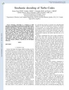
RSC2 Figure 1: Structure of a turbo encoder.
DEINT INTRODUCTION Due to the cell planning schemes and battery conservation of portable receivers, the future wireless communication systems may have to be used at very low signal-to-noise ratios (SNR). This requirement creates the necessity of using very powerful codes, capable of operating at the low SNR and good schemes for synchronization of frequency, phase and timing of the modulated signal. The codes that seem to be the most interesting are the turbo codes, a new approach to channel coding introduced in 1993, which are capable of operating very close to the Shannon limit. The behaviour of such codes is usually tested under the assumption of perfect channel knowledge and perfect synchronization. This paper looks at the effects of phase and timing mismatch on the bit error probability of turbo codes and proposes a simple timing recovery algorithm. TURBO CODES Turbo codes have been first introduced in [1] and have been a subject of an intense research ever since. They belong to a class of parallel concatenated codes - the structure of a typical turbo encoder can be seen in figure 1. It consists of two systematic recursive convolutional encoders (RSC), which are separated by a pseudo-random interleaver (INT). The output of the encoders can be additionally punctured in order to reduce the rate of the code.
yk1
MAP1
INT MAP2
xk yk2
INT
Figure 2: Structure of a turbo decoder. The simplicity of the encoder is counterbalanced, however, by a much more complicated decoder structure, which is shown in figure 2. A typical turbo decoder uses two separate Soft-In/ Soft-Out MAP decoders which are connected with a proper bit reordering by an interleaver (INT) and two deinterleavers (DEINT). The most widely used MAP algorithm is the recursive BCJR algorithm (the details of its operation are presented in [2]),which allows for relatively easy calculation of the log likelihood ratio (LLR). Unfortunately, it requires precise knowledge of the channel parameters. The most significant feature of the turbo decoder is the feed-back loop which uses the soft bit output of one decoder as additional apriori information for the second decoder, hence the name ‘turbo code’. It works iteratively, i.e. the decoding improves with consecutive iterations. there is, however, a threshold, after which additional runs of the algorithm do not decrease the number of errors.
The problem of synchronization is even more complicated when the bandwidth and energy are sparse, that is to say, no pilot signals and known training sequences may be used to recover the phase and timing position. In such a scheme, only the Non Data Aided (NDA) estimation schemes are applicable.
0
10
−1
10
−2
BER
10
TURBO CODES AND SYNCHRONIZATION
−3
10
The behaviour of turbo coding schemes when the synchronization parameters are not perfect has not received much attention yet. It has, however, a crucial impact on the performance as it will be shown in next sections.
−4
10
−5
0
0.5
1
1.5 E /N (dB) b
2
2.5
3
0
Figure 3: Bit error rate (BER) of the (031,027), rate 1/2 turbo code for block length of N=256 and after 10 decoding iterations. In figure 3 the superior performance of a simple turbo code on an AWGN channel is shown. There exist, however, drawbacks: large hardware complexity and relatively long decoding delay due to the block nature of the code and its iterative decoding scheme. SYNCHRONIZATION Good synchronization is essential in digital wireless communication. The incoming HF signal needs to be downconverted to lower frequency and sampled properly in order to minimize intersymbol interference [6]. Such conversion requires exact knowledge of signal frequency, phase and symbol period. Any mismatch in those parameters may lead to severe degradation of the system performance and increased bit error rate. The synchronization problem becomes more difficult at low symbol SNR (ES/N0), which is clearly shown by the modified Cramer-Rao bounds for the variance of the phase estimation error given by (see [5]) 1 var { θ – θˆ } > ------------------2⋅N⋅γ
(1)
All the following graphs (if not otherwise stated) were based on simulation results for the following parameters: • (031,027) turbo code with rate 1/2 • block length of N=256 • 10 decoding iterations • AWGN channel • QPSK modulation • half-raised cosine pulse (roll-off=0.3) • 10000 transmitted blocks In figure 4, one can see the performance of a turbo coding scheme when the symbol timing is not perfectly known but varies according to the gaussian distribution around the optimum value. It is clear that even moderate variance of a timing error causes severe degradation of the BER and can be attributed to the operational principle of the decoder which requires precise knowledge of the signal-to-noise ratio. When the missynchronization occurs, the given SNR is no longer valid and the decoder tends to make more decoding errors than usually (see [3]). 0
10
−1
10
−2
10
BER
10
−3
10
and for the timing error variance given by −4
1 var { ε – ε 0 } > -------------------------2⋅N⋅γ⋅ξ
10
(2)
where N is the number of symbols, γ the symbol SNR and ξ the normalized mean square bandwidth of the pulse spectrum given for root-raised cosine pulse by π2 ξ = ----- + β 2 ( π 2 – 8 ) 3
where β is a roll-off factor.
(3)
ideal CR var=0.01 var=0.03 var=0.05 var=0.07 var=0.1
−5
10
0
0.5
1
1.5 E /N (dB) b
2
2.5
3
0
Figure 4: Bit error rate of the turbo code caused by symbol timing offset (variance is normalized by the symbol period length).
0
10
−1
1
10
0.8 −2
10 BER
0.6
−3
10
−4
10
0.4
ideal CR var=0.01 var=0.03 var=0.05 var=0.07 var=0.1
0.2 0 0.5 1
−5
0
0.5
1
1.5 E /N (dB) b
2
2.5
3
0
Figure 5: Bit error rate of a turbo code caused by phase offset (variance is not normalized). Figure 5 shows similar behaviour, this time for the phase offset mismatch. In both pictures, the reference graphs of a perfectly synchronized turbo decoder and a decoder working with synchronization parameter errors given by the CramerRao bound (calculated using (1),(2) and (3)) were added for comparison (pdf was again assumed to be gaussian). It must be noted that the bound provided by the Cramer-Rao inequalities is rather loose in this SNR region and is not likely to be approached even with the most advanced synchronization techniques (see [4]).
Time offset (ε/T)
0 −0.5 −1
−0.5 Phase offset (θ/π)
Figure 6: Normalized sum of squared soft bits of the turbo decoder after one iteration.
1 0.8 BER
10
0.5
0
0.6 0.4 0.2 0 0.5
SOFT BITS OUTPUT
1 0.5
0
The turbo coding schemes use the MAP approach for detection of data. The code is decoded on a block-by-block basis, using the iterative algorithm, which produces soft bits at each iteration. The bits are subsequently fed back for the next iteration and the algorithm repeats itself. Such a scheme provides new means of synchronization by making use of the soft output and calls for the block-based synchronization instead of a symbol-by-symbol one. In figure 6 the behaviour of the soft bit output of a turbo decoder for different time and phase offsets is presented. The soft bits produced by the decoder over a decoding block were squared, added together and finally normalized by the highest value. It can be clearly seen that the maximum lies exactly in the point of perfect synchronization - there are no strong local maxima. Such a feature should render soft bit synchronization possible using some type of maximum search algorithm. Similar behaviour can be noticed with the BER graph in figure 7. Also here there is only one distinct minimum, even though the differences between the BER values are not large (in a linear scale) for a relatively wide range of synchronization offsets.
Time offset (ε/T)
0 −0.5 −1
−0.5 Phase offset (θ/π)
Figure 7: BER of the turbo decoder after ten iterations. RECEIVER STRUCTURE The proposed receiver’s structure (figure 8) attempts to move the signal processing to the digital domain as early as possible. The sampling is done by a free-running sampler and the sampled signal (generally not synchronized) is fed to the digital matched filter (DMF). It is then processed by the interpolator unit (INTP) which tries to recover proper values of the signal at the optimum sampling point by means of linear interpolation (or any other similar scheme). The signal is then phase-corrected and finally fed to the turbo decoder (TURBO) which generates soft bits used by the timing and phase estimators to generate symbol timing and phase estimates. The phase estimator can in addition be used to fine-tune the frequency synthesizer used for down conversion of the incoming HF analog signal.
analog part
LOOKUP TABLE
TIMING ESTIM.
DMF
INTP
DMF
TURBO
INTP
TURBO1
∑(
⋅ )
TURBO2
∑(
⋅ )
2
digital part FREQ. SYNTH.
PHASE ESTIM.
Figure 8: Digital receiver structure with a turbo decoder.
2
Figure 9: Timing recovery unit based on two turbo decoders (or one used in sequential manner).
TIMING ESTIMATOR 400
In figure 9 we show the proposed ad-hoc timing estimator based on the soft bit output of a turbo decoder. The timing estimator works with the following assumptions: 1. Sampling is done exactly twice per symbol - the packet is short enough for this to hold, even if the sampling clock has a small drift. 2. The phase is perfectly known prior to the timing recovery - the phase recovery algorithm is not specified in this paper and will be treated separately in the near future. 3. The timing offset lies in the range of 1 1 ε ∈ (– --- T S,--- T S) 2 2
(4)
where TS is the symbol period - in a practical system one can expect some means of external crude synchronization, i.e. by additional signalling channel. The algorithm works as follows: after sampling and filtering of the signal by the matched filter, two set of samples separated by one symbol period are fed independently to the turbo decoder which performs the standard decoding procedure for one iteration. After that, the soft bits generated for both sets are squared, added and subtracted, thus forming a metric, which is subsequently fed to the lookup table. The lookup table produces the timing estimate which is used by the interpolator to modify the set of samples using linear approximation. The new samples may be used for data detection or for improvement of the timing estimate in the next iteration. The target function stored in the lookup table is shown in the figure 10. The function has a nice monotonic behaviour, although in the region close to the optimum sampling point it is a little too flat, which may (and indeed does) cause quite large errors. Part of the future research will concentrate on finding a better function, that is to a say, a function which is linear in the wider range of the timing offset.
300 200 100 0 −100 −200 −300 −400 −0.5
0 ε/T
0.5
Figure 10: Lookup table function for SNR=3dB. PERFORMANCE The performance of the proposed timing recovery algorithm was tested and compared with the traditional ML timing estimator described in [4]. Such an ML synchronizer uses a bank of matched filters (in this case we used 50 filters) with different delays, corresponding to different timing offsets. After the initial sampling, the digitized signal is fed to those filters, which results in sample sequences of different delays. These sequences are then downsampled (so only one sample per symbol remains) and the resulting values are squared and added over the block forming a target function given by equation (5). N–1
L(ε) =
∑
zn ( ε ) 2
(5)
n=0
In the next step the resulting metrics are compared and the delay corresponding to the highest value of L chosen as the desired timing estimate. Using this estimate the linear interpolator finds new values of the incoming samples, which in turn are used for the decoding purposes.
−1
10
0.4 ML MAP
0.35 0.3 −2
10
0.25 0.2
CR ML MAP
−3
10
0.15 0.1 0.05
−4
10
0
0.5
1
1.5 Eb/N0 (dB)
2
2.5
3
Figure 11: Timing error variances of the tested synchronization schemes and the Cramer-Rao bound. 0
10
−1
10
−2
BER
10
−3
10
MAP ML ideal CR
−4
10
−5
10
0
0.5
1
1.5 Eb/N0 (dB)
2
2.5
3
0 −1
−0.5
0 ε/T
0.5
1
Figure 13: Timing error distribution of the ML and MAP synchronizers. The actual error distribution for the ML and the MAP scheme can be seen in the figure 13. The ML error distribution curve is narrower than the MAP one, but there are also large errors which occur when the initial sampling offset is close to the maximum half symbol period. It must be understood that those large errors are not cycle slips they do not cause losing of the symbol. The MAP synchronizer produces more crude estimates but they are confined to the range of offsets (-0.3TS,+0.3TS). This is a direct consequence of the large flatness of the target function in this region (a relatively small metric error causes large timing offset error) and should be easy to improve by choosing a slightly different target function. It may be also possible to combine both types of synchronizers and obtain a narrow error distribution without ML problems with large initial timing offsets.
Figure 12: BER for differently synchronized turbo codes.
CONCLUSIONS
The variances of the timing estimate produced by the proposed algorithm (MAP), the reference ML algorithm and the Cramer-Rao bound (CR) as given by equations (2) and (3) are shown in figure 11. The timing error variance provided by the proposed MAP algorithm outperforms the ML estimate for SNR larger then approximately 1.5dB. This behaviour is confirmed by figure 12 which shows the actual BER of the turbo code used together with the synchronization units described above. The MAP synchronizer achieves better results in the region of SNR>2.5dB. Also the ML synchronizer seems to reach a performance floor and the curve becomes much flatter than the one corresponding to the MAP synchronizer. For the lower SNR, the MAP scheme can be improved using more synchronization steps than just one, and/or increasing the sampling rate.
The joint synchronization and decoding of turbo codes is likely to give good results and may be the only way of successful operation in the low SNR region. As it was shown, even the simple, ad-hoc solution presented in the paper clearly outperforms traditional methods and reduces the hardware complexity by making use of the turbo decoder structure. Moreover, the tested algorithm does not use any pilot symbols although it seems probable that including even a small number of synchronization bits could increase the performance without significant reduction of the code rate. There remains, however, large room for improvement and modifications of the scheme. The research on this problem is unfortunately very scarce and there is a great number of questions still to be answered.
FUTURE PLANS The future work in this WP will try to address the following problems: 1. Theoretical analysis of the turbo code behaviour with a given phase and timing offset error distribution such analysis is likely to be rather difficult and will probably involve a lot of approximations and simplifications. 2. Development of a good joint parameter recovery algorithm - it should find the soft bits output maximum with the minimal number of additional iterations and lowest possible complexity. 3. Multi-iteration synchronization algorithms - it may be possible to increase the performance of the synchronizer when the adjustment of parameters is done after each decoding iteration. 4. Hybrid ML-MAP synchronization scheme - it may be possible to use some sort of the ML post-synchronizer together with the main MAP algorithm in order to benefit from the good performance of the ML scheme in the proximity of optimal sampling point and the MAP algorithm with larger timing offsets. 5. Influence of the sampling frequency and interpolation technique on the algorithm performance - the increased sampling rate may help construct better estimator of the timing offset and decrease the error of the linear interpolator. Also other types of interpo-
lators should be tested, 6. Synchronization for a fading channel - the algorithm should work with non-ideal knowledge of the channel and be able to combat different types of fading phenomenon. 7. Training pilot symbols - while reducing the code rate, they could be used for significant improvement of a system performance. REFERENCES [1]
[2]
[3]
[4] [5] [6]
C. Berrou, A.Glavieux, and P.Thitimajshima, “Near Shannon limit error-correcting coding and decoding: turbo codes,” ICC 1993, pp. 1064-1070. S.A.Barbulescu, Iterative Decoding of Turbo Codes and Other Concatenated Codes, PhD Dissertation, University of South Australia, 1996. T.A. Summers and S.G.Wilson, “SNR Mismatch and Online Estimation in Turbo Deciding”, IEEE Transactions on Communications, vol. 46, 1998, pp. 421-423. H.Meyr, M.Moeneclaey, and S.A.Fechtel, Digital Communication Receivers, Wiley 1998 U.Mengali, A.N.D’Andrea, Synchronization Techniques for Digital Receivers, Plenum Press 1997 J.G.Proakis, Digital Communications, McGrawHill 1995