AbstractâWe consider waveform design for multiple-input, multiple-output radar systems for the case where the signal, dur- ing propagation, undergoes phase ...
DRDC-RDDC-2013-P1
Joint Waveform Optimization and Adaptive Processing for Random-phase Radar Signals A. A. Gorji∗ , R. J. Riddolls† , Maryam Ravan∗ , Raviraj S. Adve∗
† Radar
∗ Department
of Electrical and Computer Engineering, University of Toronto Systems Section, Defence Research and Development Canada, Ottawa, Ontario, Canada
Abstract—We consider waveform design for multiple-input, multiple-output radar systems for the case where the signal, during propagation, undergoes phase perturbations. We formulate an iterative algorithm to obtain both waveform parameters and the weights of the adaptive matched filter. An example of a clutter and target model is provided to show how the optimal waveform design improves the detection performance of a random-phase radar compared to traditional waveforms.
I. I NTRODUCTION There has been much recent interest in waveform design for multiple-input, multiple-output (MIMO) radars. For example, the works in [1]–[3] find the optimal waveforms that maximize the mutual information between the received signal and target amplitude. When the resolution capability of the MIMO radar system is of interest, the transmit waveform can be designed to sharpen the radar ambiguity function [4], [5]. However, the obtained waveform does not necessarily improve the accuracy of target estimates; this, in turn, has motivated waveform design to minimize the Cramer-Rao bound [6], [7]. In the context of target detection, the signal-to-interferenceplus-noise ratio (SINR) is a well accepted design metric [8]– [11] for waveform design. In [8] the transmit waveform code is assumed to be represented by an unknown code matrix and the code design is formulated as an optimization problem with several non-convex constraints. A robust technique, using minimax optimization, was formulated in [9] for the case of unknown target parameters, such as Doppler and time delay. In [10], Friedlander optimizes the values of the discrete Fourier transform of the transmitted signal to maximize SINR. Another optimization framework based on SINR was proposed in [11] where an iterative algorithm is used to estimate the optimal waveform as well as the optimal receiver transfer function. A common theme to all these SINR-maximization approaches is the need for second order statistics. To establish realistic second-order statistics, we consider the example of a radar operating in a plasma medium. The medium is assumed to contain plasma density inhomogeneities that impart a randomization (denoted as scintillation) of the phase in the spatial and temporal domains. The phase scintillation manifests itself as an apparent angular and Doppler spreading of the signal that can be characterized by a spatial-temporal correlation function. This correlation function determines the nature of the SINR and the resulting waveform and adaptive filter optimization. A key feature of the plasma example is that well-established fluid and electromagnetic properties of
978-1-4799-2035-8/14/$31.00 ©2014 Crown
the plasma can be used to determine the nature of the spatialtemporal correlation function from first principles without the need to adopt empirical models. Specifically, we consider a class of plasma with high Reynolds number, which tends to develop turbulence structure with a characteristic Kolmogorov inverse-power law wavenumber spectrum. This paper proposes a joint waveform optimization and adaptive processing for a random-phase radar system. The signal model for our random-phase radar system is first discussed and the SINR for the given structure is derived. Afterwards, an iterative optimization algorithm is formulated to obtain both the waveform and adaptive matched filter (AMF) weights. The superiority of the new joint framework to traditional waveform design is then justified by evaluating the detection performance of the radar structure. The rest of this summary is organized as follows. Section II reviews the signal and clutter model. Based on these models, the SINR is derived in Section III and the receive adaptive weights and waveform are optimized. Section IV then presents numerical results that illustrate the gains possible using waveform optimization. Finally, Section V concludes the paper. II. S IGNAL M ODEL The radar system considered in this paper is configured in monostatic mode with 𝑁𝑇 transmitters and 𝑁𝑅 receivers that are closely-spaced in a two-dimensional space. For ease of exposition, the transmitter and receiver are assumed to be configured as uniform linear arrays aligned with the 𝑥-axis of a Cartesian coordinate system, with inter-element spacings of 𝑑𝑇 and 𝑑𝑅 , respectively. The transmitted waveform by the 𝑚-th transmitter is given by 𝐼 ∑ u𝑚 (𝑡) = C𝑚𝑖 𝑠(𝑡 − 𝑖𝑇𝑟 ), (1) 𝑖=1
where 𝐼 denotes the total number of pulses transmitted per burst, 𝑇𝑟 is the pulse-repetition interval (PRI), C denotes the transmitted code matrix that is being optimized and 𝑠(𝑡) is a fixed unit energy “template” pulse emitted by each transmitter. A. Data Model Over 𝑁𝐵 range bins, the received signal can be represented as a 𝑁𝑅 𝐼 ×𝑁𝐵 matrix Y where each column is a length-𝑁𝑅 𝐼 vector corresponding to a single range bin and is written as y = t + q + w,
(2)
����
where {t, q} denote the signal contributed by the target and clutter, and w represents additive Gaussian noise with known covariance matrix R𝑤 . Traditional models for the target generally assume a point target with freespace line-of-sight (LOS) propagation; similarly, clutter is modeled as a superposition of freespace LOS propagation from an assortment of clutter sources, e.g., [12]. For simplicity, we consider a two-dimensional radar configuration in the 𝑥𝑦 plane, with the radar signal ray path forming an angle 𝜃 with respect to the 𝑥-axis. In contrast to the freespace case, propagation in inhomogeneous media suffers from the effect of refractive index fluctuations, leading to scintillations in the signal amplitude and phase. We focus on the phase scintillation in this paper as this effect is the dominant influence on the temporal coherence (Doppler spread) and spatial coherence (angle-ofarrival spread) of the radar signal. The phase of a signal at a given point in time is equal to the integration of its spatial rate of change over the ray path: ∫ 𝑠1 𝑘(r) 𝑑𝑠, (3) 𝜙= 𝑠0
where 𝑘(r) is the radar signal wavenumber, 𝑑𝑠 is an element of arc length, and (𝑠0 , 𝑠1 ) are the ray path end points. If we suppose there are no zero-order plasma density gradients in our assumed two-dimensional plasma volume, then the rays form straight lines that can be taken as radial with respect to the radar in a system of polar coordinates (𝜌, 𝜃). Let us consider a first-order Taylor series pertubation of 𝑘(r) with respect to plasma density 𝑛, such that we can write the phase perturbation as ∫ 𝜌1 ∂𝑘(r) 𝑑𝜌, (4) 𝑛1 (r) 𝜙1 = ∂𝑛 𝜌0 where 𝑛1 is the plasma density perturbation, and (𝜌0 , 𝜌1 ) is the interval of integration in the radial coordinate. The dispersion relation for an unmagnetized plasma is given by 𝜔 2 = 𝑐2 𝑘 2 +
𝑞𝑒2 𝑛 , 𝜖 0 𝑚𝑒
(5)
where 𝜔 is the carrier frequency, 𝑐 is the speed of light, 𝑞𝑒 is the charge on an electron, 𝜖0 is the permittivity of free space, and 𝑚𝑒 is the mass of an electron. Using the dispersion relation to compute ∂𝑘(r)/∂𝑛, we arrive at ∫ 𝜌1 𝑛1 (r) 𝑑𝜌, (6) 𝜙1 = −𝑟𝑒 𝜆 𝜌0
where 𝑟𝑒 = 𝑞𝑒2 /(4𝜋𝜖0 𝑚𝑒 𝑐2 ) = 2.8 × 10⁻¹⁵ m is the classical electron radius, and 𝜆 is the radar wavelength in the plasma. The spatial-temporal autocorrelation of 𝜙1 in the assumed twodimensional geometry is given by 𝑅𝜙1 (𝑋, 𝑌, 𝑇 ) = ∫ 𝜌1 ∫ 𝜌1 2 𝑅𝑛1 (𝑋 + 𝑥 − 𝑥′ , 𝑌 + 𝑦 − 𝑦 ′ , 𝑇 ) 𝑑𝜌 𝑑𝜌′ . (7) (𝑟𝑒 𝜆) 𝜌0
𝜌0
978-1-4799-2035-8/14/$31.00 ©2014 Crown
After Fourier transforms we have 𝑆𝜙1 (𝜅𝑥 , 𝜅𝑦 , Ω) = (𝑟𝑒 𝜆)2 𝑆𝑛1 (𝜅𝑥 , 𝜅𝑦 , Ω) ∫𝜌 ∫𝜌 ′ × 𝜌01 𝜌01 𝑒𝑖(𝜅𝑥 cos 𝜃+𝜅𝑦 sin 𝜃)(𝜌−𝜌 ) 𝑑𝜌 𝑑𝜌′
= 2𝜋𝐿(𝑟𝑒 𝜆)2 𝛿(𝜅𝑥 cos 𝜃 + 𝜅𝑦 sin 𝜃)𝑆𝑛1 (𝜅𝑥 , 𝜅𝑦 , Ω), (8)
where 𝐿 = 𝜌1 − 𝜌0 is the path length, and it is observed that the Dirac delta function assures that 𝜅𝑦 = −𝜅𝑥 cot 𝜃. For a two-dimensional turbulent plasma, the Kolmogorov turbulence spectrum has a 𝜅−8/3 dependence, which we approximate as 𝜅−3 : 〈 〉 4𝜋 2 𝜅0 𝑛21 𝛿(Ω) , (9) 𝑆𝑛1 (𝜅𝑥 , 𝜅𝑦 , Ω) = 2 (𝜅0 + 𝜅2𝑥 + 𝜅2𝑦 )3/2 where 𝜅0 is the inverse scale length of the largest turbulent eddies and we have assumed no temporal structure. The spectrum is normalized as follows: ∫∫∫ 〈 2〉 1 𝑆𝑛1 (𝜅𝑥 , 𝜅𝑦 , Ω) 𝑑𝜅𝑥 𝑑𝜅𝑦 𝑑Ω. (10) 𝑛1 = (2𝜋)3 If the plasma is drifting, then temporal structure is created by the movement of spatial structure past a point in space, namely 〈 〉 4𝜋 2 𝜅0 𝑛21 𝛿(Ω − 𝜅𝑥 𝑣𝑑𝑥 − 𝜅𝑦 𝑣𝑑𝑦 ) . (11) 𝑆𝑛1 (𝜅𝑥 , 𝜅𝑦 , Ω) = (𝜅20 + 𝜅2𝑥 + 𝜅2𝑦 )3/2 By inserting this expression for 𝑆𝑛1 (𝜅𝑥 , 𝜅𝑦 , Ω) into (8) and recalling that 𝜅𝑦 = −𝜅𝑥 cot 𝜃, we can integrate out the 𝜅𝑦 coordinate so that the phase spectrum becomes 𝑆𝜙1 (𝜅𝑥 , Ω) = 〈 〉 8𝜋 3 𝜅0 𝐿 csc 𝜃(𝑟𝑒 𝜆)2 𝑛21 𝛿 (Ω − 𝜅𝑥 (𝑣𝑑𝑥 − 𝑣𝑑𝑦 cot 𝜃)) .(12) (𝜅20 + 𝜅2𝑥 csc2 𝜃)3/2 Given the phase spectrum in (12), the data cube is then crated by forming a two-dimensional sensor-pulse phase signal at each√range bin by filtering white noise through 𝐻 = IFFT ( 𝑆𝜙1 ). The resulting data cube is then convolved with the ambiguity function of the transmitted signal. B. Target Contribution The target is assumed to lie in a single far-field range bin and that it can be modeled as a point source with amplitude 𝛼𝑡 . Further, the target is located at an azimuth angle 𝜃𝑡 with respect to the receive array and Doppler frequency Ω𝑡 . In this application, the key difference from previous approaches is that the propagation through plasma media generates randomphase perturbations in the signal contributed by the target at the receiver. These perturbations must be accounted for in the design of the transmit waveform and adaptive receiver. Let 𝜙𝑡𝑖𝑛 represent the random phase perturbation at the 𝑛-th (of 𝑁𝑅 ) receiver and the 𝑖-th (of 𝐼) pulse. Based on the target model in Section II-A, after matched filtering to the transmit pulse, the (𝑖𝑛)-th entry of t can be written as: t𝑖𝑛 = 𝛼𝑡
𝑁𝑇 ∑
𝑡
C𝑚𝑖 𝑒𝑗𝜙𝑖𝑛 𝑒𝑗2𝜋Ω𝑡 𝑖𝑇𝑟 𝑒𝑗2𝜋𝑓𝑠 (𝛾𝑚+𝑛) ,
(13)
𝑚=1
where 𝛾 = 𝑑𝑇 /𝑑𝑅 , 𝑓𝑠 = 𝑑𝑅 cos(𝜃𝑡 )/𝜆 is the spatial frequency, and 𝑇𝑟 is the Pulse Repetition Interval (PRI).
����
For convenience, we define the following matrices and vectors: ∙ the length-𝐼𝑁𝑇 vector c = VEC(C) and (𝑁𝑅 𝐼𝑁𝑇 ) × ˇ = (𝑁𝑅 𝐼𝑁𝑇 ) augmented transmit code matrix as C 𝐼𝑁𝑅 ⊗ C; ∙ the Doppler vector aΩ as the length-𝐼 vector [aΩ ]𝑖 = exp(𝑗2𝜋𝑖Ω𝑡 𝑇𝑟 ). Further, define the 𝐼 × 𝐼 diagonal matrix AΩ = diag(aΩ ); ∙ based on these definitions, define two forms of a spatialtemporal matrix Θ = ˇ = Θ
a 𝑅 ⊗ AΩ ⊗ a 𝑇 , 𝑑𝑖𝑎𝑔(a𝑅 ) ⊗ AΩ ⊗ (a𝑇 )′ ,
(14) (15)
with a𝑇 and a𝑅 being the transmit and receive steering vectors, respectively. ∙ finally, define length-𝐼𝑁𝑅 vector p𝑡 such that [p𝑡 ]𝑖+𝑛𝐼 = 𝜙𝑡𝑖𝑛 , the vectorized form of the phase perturbations and the 𝐼𝑁𝑅 × 𝐼𝑁𝑅 diagonal phase perturbation matrix P𝑡 as [P𝑡 ]𝑖𝑛 = diag(p𝑡 ). Based on these definitions, the target-generated signal in (13) can be re-written in the two following forms: ˇ 𝑡, ˇ Cp (16) t = 𝛼𝑡 Θ t = 𝛼𝑡 P𝑡 Θc.
(17)
C. Clutter Contribution As seen in Section II-A, the clutter model is similar to the target model with multiple clutter rays contributing to the overall signal. Using (12), we know that the clutter-generated phase perturbations are both spatially and temporally correlated. Inspired by the signal model proposed for the target, the clutter-contributed signal can be also written as q=
𝑁𝜃 ∑
ˇ 𝑞 (𝜃𝑣 ), ˇ 𝑞 (𝜃𝑣 )Cp Θ
(18)
𝑣=1
where 𝑁𝜃 denotes the number of azimuth paths over which ˇ 𝑞 (𝜃𝑣 ) = diag(a𝑅 (𝜃𝑣 )) ⊗ the clutter signal is received, and Θ ′ AΩ,𝑞 (𝜃𝑣 ) ⊗ (a𝑇 (𝜃𝑣 )) and p𝑞 (𝜃𝑣 ) defined similarly to the corresponding terms for the target signal but for clutter azimuth angle 𝜃𝑣 . Similarly, we have AΩ,𝑞 (𝜃𝑣 ) = exp(𝑗2𝜋𝑖Ω(𝜃𝑣 )𝑇𝑟 ) where Ω(𝜃𝑣 ) denotes the mean Doppler shift of the clutter patch at azimuth angle 𝜃𝑣 . We assume that different azimuth angles contribute phase perturbations that are statistically independent. Specifically, given 𝜙𝑞𝑖𝑗 (𝜃𝑣 ) and 𝜙𝑞𝑖′ 𝑗 ′ (𝜃𝑣 ) as the perturbations generated by the 𝑣-th and 𝑣 ′ -th path, respectively, 𝐸{𝜙𝑞𝑖𝑗 (𝜃𝑣 )(𝜙𝑞 ) ∗𝑖′ 𝑗 ′ (𝜃𝑣′ )} = 0, ∀𝑣 ∕= 𝑣 ′ . Based on this assumption, we focus for now on a single ray path at azimuth angle 𝜃. Define, for an array along the x-axis, the spatial-temporal correlation of the phase perturbation as 𝑅(Δ𝑥, Δ𝑡) = 𝐸 {𝜙(𝑥, 𝑡)𝜙∗ (𝑥 + Δ𝑥, 𝑡 + Δ𝑡)} ,
(19)
where Δ𝑥 and Δ𝑡 are the spatial and temporal lag, respectively, and 𝐸{⋅} denotes expectation. The phase autocorrelation matrix R𝑝 is a (𝑁𝑅 𝐼)×(𝑁𝑅 𝐼) matrix whose (𝑖+𝑛𝐼), (𝑖′ + 𝑛′ 𝐼)-th entry is as R𝑝(𝑖+𝑛𝐼)(𝑖′ +𝑛′ 𝐼) = 𝑅(∣𝑛 − 𝑛′ ∣𝑑𝑅 , ∣𝑖 − 𝑖′ ∣𝑇𝑟 ).
978-1-4799-2035-8/14/$31.00 ©2014 Crown
Note that the clutter contribution in (18) is a nonlinear function of the phase and, therefore, further analysis is needed to obtain the autocorrelation matrix of received signals. We use the fact that the phase perturbations 𝜙𝑞𝑖𝑛 is as a twodimensional Gaussian random process. Lemma 1. Let 𝑧𝑖𝑛 = [p𝑞 ]𝑖+𝑛𝐼 = exp(𝑗𝜙𝑞𝑖𝑛 ) represent the clutter phase term in (18). The clutter phase autocorrelation matrix is a (𝐼𝑁𝑅 ) }× (𝐼𝑁𝑅 ) matrix R𝜙 = { 𝐸 (p𝑞 − 𝐸{p𝑞 )}(p𝑞 − 𝐸{p𝑞 })† with R𝜙(𝑖+𝑛𝐼)(𝑖′ +𝑛′ 𝐼)
=
𝐸 {(𝑧𝑖𝑛 − 𝑧¯𝑖𝑛 )(𝑧𝑖∗′ 𝑛′ − 𝑧¯∗ 𝑖′ 𝑛′ )} = 𝐸 {𝑧𝑖𝑛 𝑧𝑖∗′ 𝑛′ } − 𝑧¯𝑖𝑛 𝑧¯∗ 𝑖′ 𝑛′ ( ) ) )( ( 2 − 1 , (20) = exp −𝜎𝑞2 exp 𝜎(𝑖𝑛)(𝑖 ′ 𝑛′ )
2 where 𝑧¯ = 𝐸{𝑧}), 𝜎𝑞2 is the clutter variance, and 𝜎(𝑖𝑛)(𝑖 ′ 𝑛′ ) = 𝑝 ′ ′ R (∣𝑛 − 𝑛 ∣𝑑𝑅 , ∣𝑖 − 𝑖 ∣𝑇𝑟 ).
The autocorrelation matrix of the clutter signal given in (18) for a clutter ray from azimuth angle 𝜃 can be then written as R𝑞 (𝜃) = Φ(𝜃)R𝜙 (Φ(𝜃))† ,
(21)
ˇ ˇ 𝑞 (𝜃)C. with Φ(𝜃) = Θ Finally, for the more practical case that the clutter is received over 𝑁𝜃 > 1 rays and using the statistical independence of different rays, we have R𝑞 =
𝑁𝜃 ∑
R𝑞 (𝜃𝑣 ),
(22)
𝑣=1
where each individual R𝑞 (𝜃𝑣 ) is given by (21). III. J OINT O PTIMIZATION OF S IGNAL - TO -I NTERFERENCE - PLUS -N OISE R ATIO At the receive array the signals received within each range bin are adaptively combined to maximize the SINR. Detection or localization decisions are then made on the filter output. Denoting as h the length-𝑁𝑅 𝐼 vector of adaptive weights, the SINR is given by } { 𝐸 ∣h† t∣2 . (23) SINR = 𝐸 {∣h† q∣2 } + 𝐸 {∣h† w∣2 } Note that the target and, importantly, clutter signals, t and q, are functions of the transmit code vector c. We are interested in jointly designing the unknown adaptive filter weight vector h and transmit signal c under a constraint on the total transmitted power. This optimization problem can be formulated as follows: {c𝑜 , h𝑜 } arg maxh,c SINR, (24) such that ∣∣c∣∣2 ≤ 1. The cost function in (24) is nonlinear and non-convex with respect to the joint optimization variables [c† h† ]† . Globally optimal solutions are, therefore, impossible to come by and here we propose an iterative approach in which the linear weight vectors h and input signal vector c are obtained individually.
����
A. Optimization of Adaptive Weights In optimizing for the adaptive weights, we assume the transmit waveform, defined by c, is fixed. For convenience, the formulation in (16) is used to optimize the adaptive weights h. The SINR can be then written as follows: SINR =
∣𝛼𝑡 ∣2 h† 𝝆𝑐,𝑡 h , h† 𝝆𝑐,𝑞,𝑤 h
(25)
where the subscripts 𝑡 and 𝑞 refer to the target and interference (clutter and noise) respectively, and 𝜌𝑐,𝑡 and 𝜌𝑐,𝑞,𝑤 are two known matrices that are functions of target and clutter parameters. Here, 𝝆𝑐,𝑡
=
ˇ † (Θ ˇ 𝜙 (C) ˇ 𝑡 CR ˇ 𝑡 )† , Θ 𝑡
𝝆𝑐,𝑞,𝑤
=
R𝑐 + R 𝑤
=
𝑁𝜃 ∑
(26)
ˇ 𝜙 (𝜃𝑣 )(C) ˇ † (Θ ˇ 𝑞 )† (𝜃𝑣 ) + R𝑤 , (27) ˇ 𝑞 (𝜃𝑣 )CR Θ 𝑞
𝑣=1
ˇ 𝑞 (𝜃𝑣 ) and R𝜙𝑞 (𝜃𝑣 ) are calculated using (15) and (20), where Θ respectively, for each clutter azimuth angle 𝜃𝑣 . In addition, R𝑤 denotes the covariance matrix of the additive noise. The optimal weight vector (h𝑜 ), for a given transmit code c, can be then found by maximizing the cost function in (25). A more stable approach is to use the Cholesky factorization of 𝝆𝑐,𝑞,𝑤 . Defining L𝑐,𝑞,𝑤 as the Cholesky factor of 𝝆𝑐,𝑞,𝑤 where 𝝆𝑐,𝑞,𝑤 = L𝑐,𝑞,𝑤 (L𝑐,𝑞,𝑤 )† , the following lemma presents a framework for finding the optimal solution of the liner weights: Lemma 2. The optimal solution of the problem in (25) is: ]† ( [ −1 ]† ) [ −1 , (28) 𝒫 [L ] 𝝆 h𝑜 = L−1 𝑐,𝑞,𝑤 𝑐,𝑡 L𝑐,𝑞,𝑤 𝑐,𝑞,𝑤 where 𝒫(A) corresponds to the principal component of matrix A. B. Waveform Optimization The second step within the iterative algorithm reverses this to find the optimal waveform given the adaptive weights h. In this case, using the alternate signal model in (17), the SINR can be written as SINR = ∣𝛼𝑡 ∣2
c† Ωℎ,𝑡 c
†
c† Ωℎ,𝑐 c + (h) R𝑤 h
.
(29)
where Ωℎ,𝑡 and Ωℎ,𝑐 are known-structure matrices function of target and clutter parameters, respectively. The waveform design can be now reformulated as the following optimization problem: arg maxc SINR, {c𝑜 } = (30) such that = ∣∣c∣∣2 ≤ 1. It was shown in [11] that, within a scale factor, the above optimization problem leads to the same solution as the following unconstrained SINR-maximization {c𝑜 } = arg max c
c† Ωℎ,𝑡 c . c† Ωℎ,𝑐 c + (h)† R𝑤 h.c† c
978-1-4799-2035-8/14/$31.00 ©2014 Crown
(31)
If c𝑜∗ is a solution obtained for this unconstrained problem, the final solution is c𝑜 = c𝑜∗ /∣∣c𝑜∗ ∣∣. The cost function in (31) can be simplified into the following form: c† Ωℎ,𝑡 c , (32) SINR = ∣𝛼𝑡 ∣2 † c Ωℎ,𝑐,𝑤 c with Ωℎ,𝑐,𝑤 = Ωℎ,𝑐 + (h)† R𝑤 hI𝑁𝑅 𝐼 and solution obtained in a manner similar to the optimization problem for the knownwaveform case. Define Vℎ,𝑐,𝑤 as the Cholesky factor of Ωℎ,𝑐,𝑤 . Now, using lemma 2 the optimal waveform is found as follows: ]† ( [ ]† ) [ −1 −1 −1 . (33) 𝒫 [Vℎ,𝑐,𝑤 ] Ωℎ,𝑡 Vℎ,𝑐,𝑤 c𝑜∗ = Vℎ,𝑐,𝑤 The final waveform is then obtained by normalizing the solution obtained. C. Overall Joint Optimization Algorithm The overall optimization algorithm is as follows: 1) Given the phase PSD for the clutter and target, calculate the autocorrelation matrices R𝜙𝑡 and R𝜙𝑞 (𝜃𝑣 ) where 𝑣 = 1, ⋅ ⋅ ⋅ , 𝑁𝜃 and 𝑁𝜃 denotes the number of clutter rays. 2) Based on the target and clutter parameters, compute the ˇ 𝑡 , Θ𝑞 (𝜃𝑣 ) and Θ ˇ 𝑞 (𝜃𝑣 ). spatial-temporal matrices Θ𝑡 , Θ 𝜙 ˇ † ˇ † ˇ ˇ 3) Initialize matrices 𝝆𝑐,𝑡 = Θ𝑡 CR𝑡 (C) (Θ𝑡 ) and ∑𝑁 𝜃 ˇ ˇ 𝜙 (𝜃𝑣 )(C) ˇ † (Θ ˇ 𝑞 )† (𝜃𝑣 ) + R𝑤 . 𝝆𝑐,𝑞,𝑤 = 𝑣=1 Θ𝑞 (𝜃𝑣 )CR 𝑞 4) Find the Cholesky factor of 𝝆𝑐,𝑞,𝑤 as L𝑐,𝑞,𝑤 . 5) Calculate the( optimal filter weight using (33) by h𝑜 = [ −1 ]† [ −1 ]† ) −1 L𝑐,𝑞,𝑤 𝒫 [L𝑐,𝑞,𝑤 ] 𝝆𝑐,𝑡 L𝑐,𝑞,𝑤 . 6) Form the new matrix H𝑜 = diag(h𝑜 ). 7) Initialize new matrices Ωℎ,𝑡 = Θ†𝑡 H𝑜 R𝜙𝑡 (H𝑜 )† Θ𝑡 ∑𝑁𝜃 † and Ωℎ,𝑐,𝑤 = 𝑣=1 Θ𝑞 (𝜃𝑣 )H𝑜 R𝜙𝑞 (𝜃𝑣 )(H𝑜 )† Θ𝑞 (𝜃𝑣 ) + 𝑜 † 𝑜 (h ) R𝑤 h I𝑁𝑅 𝐼 . 8) Let Vℎ,𝑐,𝑤 represent the Cholesky factor of Ωℎ,𝑐,𝑤 . 9) Using (33), set ( ]† [ ]† ) [ −1 −1 −1 as the 𝒫 [Vℎ,𝑐,𝑤 ] Ωℎ,𝑡 Vℎ,𝑐,𝑤 c𝑜∗ = Vℎ,𝑐,𝑤 optimal solution for the modified optimization problem. 10) Calculate c𝑜 = c𝑜∗ /∣∣c𝑜∗ ∣∣ as the optimal waveform. 11) Repeat steps 2)-10) until convergence, defined as a negligible change in the resulting SINR. IV. N UMERICAL R ESULTS We consider a scenario with a single target at an azimuth of 70∘ and Doppler of 1/6 of the pulse repetition frequency. There are 4 transmit antennas and 4 receive antennas, placed at half-wavelength spacing. The waveform consists of a coherent burst of 𝐼 = 36 pulses. In simulating and modeling distributed clutter, an azimuth angle step of 𝛿𝜃𝑞 = 1∘ is used. We use the clutter-to-noise Ratio (CNR) to characterize the power of the incoming clutter in the receiver. The additive noise is a circularly symmetric complex Gaussian random variable with unit variance. The performance of the waveform design framework, and the benefits of waveform design, is now evaluated by analysing
����
θ = 70, CNR = 50 (dB)
θt = 70, α = 20 (dB)
t
1
20
θ˜c = 30 30 ≤ θ˜c ≤ 40
0
0.9
30 ≤ θ˜c ≤ 50 Probability of Detection
Beam Pattern (dB)
0.8
−20
−40
−60
0.7
0.6
0.5
−80 0.4
−100
Optimal Code Hadamard Code −12
10
−120
−10
10
−8
10
−6
10
−4
10
−2
0
10
10
Probability of False Alarm
0
10
20
30
40
θ
50
60
70
80
90
Fig. 2. Fig. 1. The beampattern of the optimal waveform for the single-ray clutter and two different distributed clutter cases.
ROC curves for optimal waveform and Hadamard code designs.
1
0.9
0.8
where 𝐹𝜒22 (⋅) denotes the 𝜒2 Cumulative Distribution Function (CDF) with two degrees of freedom. Figure 2 plots the radar receiver operative characteristic (ROC) curve, comparing the performance of the optimized waveform with that of using a Hadamard code. The clutter is distributed over the span of 30∘ ≤ 𝜃˜𝑞 ≤ 50∘ . Again, both schemes use adaptivity on receive and the improvements are due to optimizing the transmit waveform. The huge improvements in detection performance are evident, especially at the lower probabilities of false alarm. For example, for 𝑃𝑓 𝑎 = 10−6 , the optimal waveform provides a detection rate of 96.5% while the Hadamard code only provides a 58.5% detection rate. Figure 3 plots the detection probabilities as a function of target amplitude (𝛼), again comparing the performance of the optimal waveform and Hadamard code. For comparison, the
978-1-4799-2035-8/14/$31.00 ©2014 Crown
0.7
Probability of Detection
the beampattern of the optimal code. Figure 1 shows the performance of the joint waveform-receiver adaptive process in the practical case of distributed clutter. The figure plots the adapted beampattern for a single clutter ray (𝜃𝑞 = 30∘ ) and two cases of distributed clutter (30∘ ≤ 𝜃˜𝑞 ≤ 40∘ and 30∘ ≤ 𝜃˜𝑞 ≤ 50∘ ). As before, the target is at 𝜃𝑡 = 70∘ . Clearly, the algorithm is able to adapt to the clutter by placing broad null in the required angular region. The penalty for placing a broad null is also evident in the reduced gain on the target. The ability to place a null in direction of the clutter improves detection performance. We now compare the detection performances of the waveform optimization and fixedwaveform schemes. In each case, assuming Gaussian signals, the probability of detection (𝑃𝐷 ) is related to probability of false alarm (𝑃𝑓 𝑎 ) as ) ( −1 𝐹𝜒2 (1 − 𝑃𝑓 𝑎 ) 2 𝑃𝐷 = 1 − 𝐹𝜒22 , (34) 1 + SINR
0.6
0.5
0.4
0.3
0.2 Optimal (single−ray) Hadamard (single−ray) Optimal (distributed clutter) Hadamard (distributed clutter)
0.1
0
0
5
10
15
20
25
30
Target Amplitude (dB)
Fig. 3. Probability of detection versus target amplitude for optimal waveform and Hadamard code designs.
detection curves were obtained for two cases; one with singleray clutter assumption and the other with distributed clutter where 30∘ ≤ 𝜃˜𝑞 ≤ 50∘ . In both cases, the CNR is set to 50dB. The improved detection performance is again clear, especially in the case of distributed clutter. The figure also illustrates the performance penalty in nulling distributed clutter. The results in Fig. 3 show that using a fixed transmission code is more sensitive to the structure of the clutter whereas optimizing the waveform makes the detection performance more robust. As expected, at very high, likely impractically high, SNR levels the performance gap is eliminated. Our final set of results focus on how the optimal waveform design improves Doppler frequency estimates as compared to non-optimal waveforms. In this example, the transmitters send 𝐼 = 36 pulses per coherent pulse interval leading to 36 Doppler resolution cells. Doppler data are now generated for the optimal waveform, Hadamard code and random code. Assuming CNR = 30dB, 𝛼 = 14dB and the distributed clutter case with 30∘ ≤ 𝜃𝑞 ≤ 50∘ , Figure 4 plots the received
����
power in different Doppler cells for all three transmission schemes. The improved Doppler discrimination using the optimal waveform is clear. The Doppler power spectrum for the optimal waveform has a clear peak at the target Doppler frequency (Ω𝑡 = PRF/6). Although the Hadamard code also shows maximum power around the same Doppler cell that was caught by the optimal waveform, its power is still 4dB lower than the maximum power achieved by the optimal code. The Hadamard code also leads to spurious Doppler peaks. Finally, unlike two aforementioned schemes, the random code fails to detect the true Doppler frequency as the maximum power occurs at incorrect Doppler frequencies.
Power (dB)
Optimal 30 20 10
0 −PRF/2
0
PRF/2
Doppler (Hz)
Power (dB)
Hadamard 12 10 8
6 −PRF/2
0
PRF/2
Doppler (Hz)
[4] C. Y. Chen and P. P. Vaidyanathan, “MIMO radar ambiguity properties and optimization using frequency-hopping waveforms,” IEEE Transactions on Signal Processing, vol. 56, no. 12, pp. 5296–5936, September 2008. [5] J. Zhang, H. Wang, and X. Zhu, “Adaptive waveform design for separated transmit/receive ULA-MIMO radar,” IEEE Transactions on Signal Processing, vol. 58, no. 9, pp. 4936–4942, September 2010. [6] J. Li, l. Xu, P. Stoica, K. W. Forsythe, and D. W. Bliss, “Range compression and waveform optimization for mimo radar: A cramer-rao bound based study,” IEEE Transactions on Signal Processing, vol. 56, no. 1, pp. 218–232, January 2008. [7] S. Gogineni and A. Nehorai, “Frequency-hopping code design for mimo radar estimation using sparse modeling,” IEEE Transactions on Signal Processing, vol. 60, no. 6, pp. 3022–3035, June 2012. [8] A. De Maio, S. De Nikola, Y. Huang, D. P. Palomar, S. Zhang, and A. Farina, “Code design for radar STAP via optimization theory,” IEEE Transactions on Signal Processing, vol. 58, no. 2, pp. 679–695, February 2010. [9] A. De Maio, Y. Huang, M. Piezzo, S. Zhang, and A. Farina, “Design of optimized radar codes with a peak to average power ratio constraint,” IEEE Transactions on Signal Processing, vol. 59, no. 6, pp. 2683–2697, June 2011. [10] B. Friedlander, “Waveform design for MIMO radars,” IEEE Transactions on Aerospace and Electronic Systems, vol. 43, no. 3, pp. 1227–1238, June 2007. [11] C. Y. Chen and P. P. Vaidyanathan, “MIMO radar waveform optimization with prior information of the extended target and clutter,” IEEE Transactions on Signal Processing, vol. 57, no. 9, pp. 3533–3544, September 2009. [12] J. Ward, “Space-time adaptive processing for airborne radar,” MIT Linclon Laboratory, Tech. Rep. F19628-95-C-0002, December 1994.
Power (dB)
Random 25 20 15
10 −PRF/2
0
PRF/2
Doppler (Hz)
Fig. 4. The received power in different Doppler cells for the optimal waveform, Hadamard code and random signal.
V. C ONCLUSIONS This paper has proposed a technique for the joint design of the waveforms and adaptive processor in a radar system. Using the model for the phase perturbations to derive related signal and clutter models, the transmitted waveform and matchedfilter weights are optimized to maximize the output SINR of the system. Importantly, and unlike some previous approaches, the impact of the transmitted waveform is accounted for in modeling the clutter. Finally, we present simulation results to illustrate the performance gains of the optimal waveform design over other non-optimal waveform techniques. R EFERENCES [1] A. Lesham, O. Naparstek, and A. Nehorai, “Information theoretic adaptive radar waveform design for multiple extended targets,” IEEE Journal of Selected Topics in Signal Processing, vol. 1, no. 1, pp. 42– 55, June 2007. [2] S. Sen and A. Nehorai, “OFDM mimo radar with mutual-information waveform design for low grazing angle tracking,” IEEE Transactions on Signal Processing, vol. 58, no. 6, pp. 3152–3162, June 2010. [3] B. Tang, J. Tang, and Y. Peng, “MIMO radar waveform design in colored noise based on information theory,” IEEE Transactions on Signal Processing, vol. 58, no. 9, pp. 4684–4697, September 2010.
978-1-4799-2035-8/14/$31.00 ©2014 Crown
����