Int. J. Communications, Network and System Sciences, 2009, 7, 669-674 doi:10.4236/ijcns.2009.27077 Published Online October 2009 (http://www.SciRP.org/journal/ijcns/).
Q-Learning-Based Adaptive Waveform Selection in Cognitive Radar Bin WANG, Jinkuan WANG, Xin SONG, Fulai LIU Northeastern University, Shenyang, China Email:
[email protected] Received June 11, 2009; revised August 12, 2009; accepted September 20, 2009
ABSTRACT Cognitive radar is a new framework of radar system proposed by Simon Haykin recently. Adaptive waveform selection is an important problem of intelligent transmitter in cognitive radar. In this paper, the problem of adaptive waveform selection is modeled as stochastic dynamic programming model. Then Q-learning is used to solve it. Q-learning can solve the problems that we do not know the explicit knowledge of statetransition probabilities. The simulation results demonstrate that this method approaches the optimal waveform selection scheme and has lower uncertainty of state estimation compared to fixed waveform. Finally, the whole paper is summarized. Keywords: Waveform Selection; Q-Learning; Space Division; Cognitive Radar
1. Introduction Radar is the name of an electronic system used for the detection and location of objects. Radar development was accelerated during World War Ⅱ. Since that time it has continued such that present-day systems are very sophisticated and advanced. Cognitive radar is an intelligent form of radar system proposed by Simon Haykin and it has many advantages [1]. However, cognitive radar is only an ideal framework of radar system, and there are many problems need to be solved. Adaptive waveform selection is an important problem in cognitive radar, with the aim of selecting the optimal waveform and tracking targets with more accuracy according to different environment. In [2], it is shown that tracking errors are highly dependent on the waveforms used and in many situations tracking performance using a good heterogeneous waveform is improved by an order of magnitude when compared with a scheme using a homogeneous pulse with the same energy. In [3], an adaptive waveform selective probabilistic data association algorithm for tracking a single target in clutter is presented. The problem of waveform selection can be thought of as a sensor scheduling problem, as each possible waveform provides a different means of measuring the environment, and related works have been examined in [4,5]. In [6], radar waveform selection algorithms for tracking accelerating targets are considered. In [7], genetic algorithms are used to perform waveform selection Copyright © 2009 SciRes.
utilizing the autocorrelation and ambiguity functions in the fitness evaluation. In [8], Incremental Pruning method is used to solve the problem of adaptive waveform selection for target detection. The problem of optimal adaptive waveform selection for target tracking is also presented in [9]. In this paper, the problem of adaptive waveform selection in cognitive radar is viewed as a problem of stochastic dynamic programming and Q-learning is used to solve it.
2. Division in Radar Beam Space The most important parameters that a radar measures for a target are range, Doppler frequency, and two orthogonal space angles. However, in most circumstances, angle resolution can be considered independently from range and Doppler resolution. We may envision a radar resolution cell that contains a certain two-dimensional hypervolume that defines resolution. Figure 1 is abridged general view of range and Doppler. Range resolution, denoted as ΔR, is a radar metric that describes its ability to detect targets in close proximity to each other as distinct objects. Radar systems are normally designed to operate between a minimum range Rmin, and maximum range Rmax. Targets seperated by at least ΔR will be completely resolved in range. Radars use Doppler frequency to extract target radial velocity (range rate), as well as to distinguish moving and stationary
IJCNS
B. WANG ET
670
AL.
with an expected frequency shift v0 has an impulse response h(t ) s* (t )e j 2 0t
(5)
The output is given by
x(t ) s ( t )e j 2 0 ( t ) r ( )d
where v0 is an expected frequency shift. The baseband received signal will be modeled as a return from a Swerling target:
Figure 1. A closing target.
targets or objects such as clutter. The Doppler phenomenon describes the shift in the center frequency of an incident waveform. In general, a waveform can be tailored to achieve either good Doppler or good range resolution, but not both simultaneously. So we need to consider the problem of adaptive waveform scheduling. The basic scheme for adaptive waveform scheduling is to define a cost function that describes the cost of observing a target in a particular location for each individual pulse and select the waveform that optimizes this function on a pulse by pulse basis. We make no assumptions about the number of targets that may be present. We divide the area covered by a particular radar beam into a grid in range-Doppler space, with the cells in range indexed by t=1,…,N and those in Doppler indexed by v=1,…,M. There may be 0 target, 1 target or NM targets. So 0 1 2 NM 1 NM CNM CNM CNM ... CNM CNM 2 NM
We define
(2)
bxx is the measurement probability where
bxx (ut ) P (Yt 1 x | X t x, ut )
x(t ) s ( t )r ( )d
(4)
In the radar case, the return signal is expected to be Doppler shifted, then the matched filter to a return signal Copyright © 2009 SciRes.
(7)
where s (t , , d ) s (t )e j 2 d t is a delayed t and Doppler-shifted vd replica of the emitted baseband complex envelope signal s(t); I is a target indicator. A approaches a complex Gassian random variable with zero mean and variance 2 A2 . We assume n(t) is complex white Gaussian noise independent of A, with zero mean and variance 2N0. At time t the magnitude square of the output of a filter matched to a zero delay and a zero Doppler shift is
2
x(t )
t
0
r ( ) s ( t ) d
2
(8)
When there is no target r (t ) v(t )
(9)
So 0
x( 0 ) n( ) s ( 0 )d
(10)
0
The random variable x( 0 ). is complex Gaussian, with zero mean and variance given by
02 E x( 0 ) x ( 0 ) 2 N 0
(11)
ξ is the energy of the transmitted pulse. When target is present r (t ) As (t )e j 2 d t I n(t )
(12)
0
x( 0 ) As ( )e j 2 d n( ) s ( 0 )d (13) 0
This random variable is still zero mean, with variance given by 12 E x( 0 ) x ( 0 )
(3)
Assume the transmitted baseband signal is s(t), and the received baseband signal is r(t). The matched filter is the one with an impulse response h(t)=s*(–t), so an output process of our matched filter is
r (t ) As (t )e j 2 d t I n(t )
(1)
The number of possible scenes or hypotheses about the radar scene is 2NM. Let the space of hypotheses be denoted by X. The state of our model is Xt=x where x∈X. Let Yt be the measurement variable. Let ut be the control variable that indicates which waveform is chosen at time t to generate measurement Yt+1, where ut∈U. The probability of receiving a particular measurement Xt=x will depend on both the true, underlying scene and on the choice of waveform used to generate the measurement. We define axx is state transition probability where axx P ( xt 1 x | xt x)
(6)
02 (1
2 A2 2
02
(14)
A( 0 , 0 ))
A(t,v)is ambiguity function, given by A( , )
1 2
s ( ) d
s ( ) s ( )e
2
j 2
d
2
(15)
Recall that the magnitude square of a complex Gaussian random variable x ~ N (0, i2 ) is exponentially IJCNS
B. WANG ET
distributed, with density given by 1
y x2 ~
e
2 i2
1
D
2 02
Pf
e
y
T
2 i2
V (p(0)) max E[ t R (p t , ut )]
(16)
x 2 02
671
also the solution of
We consequently have that the probability of false alarm Pf is given by
AL.
dx e
D 2 02
(17)
where Pt is the conditional density of the state given the measurements and the controls and P0 is the a priori probability density of the scene. P is a sufficient statistic for the true state Xt. So we need to solve the following problem T
max E[ t R (p t , ut )]
And the probability of detection Pd by Pd
1
e
x 2 12
dx e
D
2 02 (1
2 A2 2
02
A ( 0 , 0 ))
(18)
2 In the case when a target is present in cell ( , ) , assuming its actual location in the cell has a uniform distribution 2 1
D
D
Pd
1 A
(
a ,a A )
e
2 02 (1
2 A2 2
02
(22)
t 0
A ( 0 , 0 ))
d a d a (19)
where A is the resolution cell centred on (t,v) with volume |A|.
(23)
t 0
The refreshment formula of Pt is given by pt 1
BAp t 1 ' LApt
(24)
where B is the diagonal matrix with the vector (bxx (ut )) the non-zero elements and 1 is a column vector of ones. A is state transition matrix. If we wanted to solve this problem using classical dynamic programming, we could have to find the value function Vt (pt ) using Vt (p t ) max( Rt (p t , ut ) E{Vt 1 (pt 1 ) | pt }) (25) ut
It can also be written in probability form
3. Q-Learning-Based Stochastic Dynamic Programming
Vt (pt ) max( Rt (pt , ut ) P (p p t , ut )Vt 1 (p)) (26) ut
A target for which measurements are to be made will fall in a resolution cell. Another target, conceptually, does not interfere with measurements on the first if it occupies another resolution cell different from the first. Thus, conceptually, as long as each target occupies a resolution cell and the cells are all disjoint, the radar can make measurements on each target free of interference from others. Define {u0 , u1 ,..., uT } where T=1 is the maximum number of dwells that can be used to detect and confirm targets for a given beam. Then is a sequence of waveforms that could be used for that decision process. We can obtain different according to different environment in cognitive radar. Let T
Vt ( X t ) E[ R( X t , ut )] t
p P
However, in radar scene, explicit knowledge of target state-transition probabilities are unknown. So directly using Bellman’s dynamic programming is very hard. The Q-leaning algorithm is a direct approximation of Bellman’s dynamic programming, and it can solve the problem that we do not know explicit knowledge of state-transition probabilities. For this reason, Q-learning is very suitable to be used in the problem of adaptive waveform selection in cognitive radar. We define a Q-factor in our problem. For a state-action pair (pt , ut ) , Q (p t , ut )
P(p p , u )[ R (p p , u ) V t
p P
(21)
t 0
However, knowledge of the actual state is not available. Using the method of [10], we can obtain that the optimal control policy that is the solution of (21) is Copyright © 2009 SciRes.
t
t 1
t
]
(27)
Vt * max Q(p t , ut )
(20)
T
V ( X t ) max E[ t R ( X t , ut )]
t
According to (26), (27) we can derive (28)
ut
t 0
where R(Xt,ut) is the reward earned when the scene Xt is observed using waveform ut and γ is discount factor. Then the aim of our problem is to find the sequence that satisfies
t
The above establishes the relationship between the value function of a state and the Q-factors associated with a state. Then it should be clear that, if the Q-factors are known, one can obtain the value function of a given state from above fomula. So Q form of Bellman equation is Q(p t , ut )
P(p p , u )[ R (p p , u ) max Q(p
p P
t
t
t
t
t
ut 1
t 1
, ut 1 )]
(29)
IJCNS
B. WANG ET
672
Let us denote the ith independent sample of a random variable X by Si and the expected value by E(X). Xn is the estimate of X in the n th iteration. So n
E ( X ) lim
s
Xn
s
(30)
n
n n
i
i 1
i
i 1
(31)
n
We can derive X n 1 (1 n 1 ) X n n 1 s n 1
(32)
where
n 1
1 n 1
AL.
4. Simulation In this section, we make three experiments. In order to explain the necessity of waveform selection, we make the curve of measurement probability versus SNR of three waveforms. Curve of uncertainty of state estimation demonstrates validity of our proposed algorithm. We also plot the figure of Q value space versus state and waveform. We consider a simple situation. The state space is 4× 4. We consider 5 different waveforms where for each waveform u, and each hypotheses for the target x , the distribution of x is given in Table 1. The discount factor γ=0.9. State transition matrix A is given by 0.96 0.01 A 0.02 0.01
(33)
So Q(p t , ut ) E[ Rt (p pt , ut ) max Q(pt 1 , ut 1 )] (34) ut 1
where E is the expectation operator. We could use this scheme in a simulator to estimate the same Q-factor. Using this algorithm, Equation (29) becomes: Q n 1 (pt , ut ) (1 n 1 )Q n (pt , ut ) n 1[ Rt (p pt , ut ) max Q n (pt 1 , ut 1 )]
(35)
ut 1
Obviously, we do not have the transition probabilities in it. Our Q-learning algorithm is as follows: Step 1. Initialize the Q-factors to 0. Set n=1. Step 2. For t=0,1,…T,do step 3-step 6. Step 3. Simulation action ut. Let the curren state be Pt, and the next state be Pt+1. Step 4. Find the decision using the current Q-factors: ut arg max Qtn 1 (p tn , ut )
R (p, u ) p ' p 1
The formula E(–R) can be considered as the uncertainty in the state estimation. In other words, it can be considered as the tracking errors. Figure 2 is curve of measurement probability versus SNR of three waveforms. From this curve we can see that with the same SNR, different waveforms correspond to different measurement probability. Generally speaking, the waveform with wide pulse duration corresponds to high measurement probability. From this point of view, the waveform with wide pulse duration is better. However, wide pulse duration means large energy of the transmitted pulse. So we should improve measurement 1
(36)
Step 5. Update Q(Pt,ut) using the following equation: (pt , ut ) (1
)Q (pt , ut )
n 1[ Rt (p pt , ut ) max Q n (pt 1 , ut 1 )]
(37)
ut 1
Step 6. Find the next state: pt 1
BAp t 1 ' BApt
(38)
d (pt ) arg max Q(p t 1 , ut 1 ) ut
The policy generated by the algorithn is dˆ . Stop.
0.7 0.6 0.5 0.4 0.3 0.2
Step 6. Increment n. If n