Feb 4, 2018 - ... in the diagram. arXiv:1802.01095v1 [cond-mat.mes-hall] 4 Feb 2018 .... mean escape time Ï for the Lévy statistics reads [45, 46] Ï (α, D) = C α.
Josephson-based threshold detector for Lévy distributed fluctuations Claudio Guarcello,1, 2 Davide Valenti,3 Bernardo Spagnolo,3, 2, 4 Vincenzo Pierro,5 and Giovanni Filatrella6
arXiv:1802.01095v1 [cond-mat.mes-hall] 4 Feb 2018
1
NEST, Istituto Nanoscienze-CNR and Scuola Normale Superiore, Piazza S. Silvestro 12, I-56127 Pisa, Italy 2 Radiophysics Dept., Lobachevsky State University, 23 Gagarin Ave., 603950 Nizhniy Novgorod, Russia 3 Dipartimento di Fisica e Chimica, Group of Interdisciplinary Theoretical Physics, Università di Palermo and CNISM, Unità di Palermo, Viale delle Scienze, Edificio 18, 90128 Palermo, Italy 4 Istituto Nazionale di Fisica Nucleare, Sezione di Catania, Via S. Sofia 64, I-95123 Catania, Italy 5 Dept. of Engineering, University of Sannio, Corso Garibaldi 107, I-82100 Benevento, Italy 6 Dep. of Sciences and Technologies and Salerno unit of CNISM, University of Sannio, Via Port’Arsa 11, Benevento I-82100, Italy We propose a threshold detector for Lévy distributed fluctuations based on a Josephson junction. The Lévy noise current added to a linearly ramped bias current results in clear changes in the distribution of switching currents out of the zero-voltage state of the junction. We observe that the analysis of the cumulative distribution function of the switching currents supplies information on both the characteristics shape parameter α of the Lévy statistics and the intensity of the fluctuations. Moreover, we discuss a theoretical model which allows from a measured distribution of switching currents to extract characteristic features of the Lévy fluctuations. In view of this results, this system can effectively find an application as a detector for a Lévy signal embedded in a noisy background.
Introduction. – A current-biased Josephson junction (JJ) represents a natural threshold detector for current fluctuations, inasmuch as it is a metastable system operating on an activation mechanism. Actually, the behaviour of a JJ can be depicted as a particle, representing the superconducting phase difference ϕ across the JJ, in a cosine “washboard” potential with friction [1, 2], see Fig. 1(a). In this picture, the slope of the washboard potential is given by the injected current, and the dynamics of the phase is described by the resistively and capacitively shunted junction (RCSJ) model. The equivalent particle remains near a washboard minimum (correspondingly, the JJ is in the zero-voltage metastable state) until the direct bias current exceeds a critical value, or a fluctuation sets the phase ϕ in motion along the potential. Indeed, a current fluctuation instantaneously tilts the potential, and a noise-induced escape from a minimum can occur. In correspondence of the escape a voltage develops, as the voltage is related to the velocity of the phase particle. Shortly, if a JJ is set in the fundamental zero-voltage state, noise can cause a passage from this zero-voltage state to the finite voltage “running” state. The statistics of these passages can be exploited to reveal the features of the noise. After early suggestions [3–5], several proposals for concrete experimental setup of Josephson-based noise detectors have been put forward [6–12]. A scheme to detect the Poissonian character of the charge injection in an underdamped JJ, based on the analysis of the thirdorder moment of the electrical noise, was proposed in Ref. [3] and a scheme to detect the fourth-order moment of the noise was discussed in Ref. [4]. A threshold detector based on an array of overdamped JJs for the direct measurement of the full counting statistics, through rare over-the-barrier jumps induced by current fluctuations,
was suggested in Ref. [5]. Alternatively, in the Coulomb blockade regime, the sensitivity of the JJ conductance to the non-Gaussian character of the applied noise was demonstrated [13, 14]. Most proposals make use of the
Ib(t)
Ic
U = U0[1-cos(φ)-ibφ]
t
JJ
(a)
t
C
R
IN(t)
V V(t)
(c) ΔU Δx
(b)
FIG. 1. (a) The phase particle in a potential minimum of the tilted washboard potential U . The barrier height, ∆U , and the distance between the minimum and maximum of the potential, ∆x, are also shown. (b) ϕ trajectories in the noisy driven case when the Lévy stochastic term dominates. (c) Simplified equivalent circuit diagram for the RCSJ model. The linearly ramped bias current, Ib (t), and the noise current, IN (t), of the JJ are included in the diagram.
2 information content of higher moments, beyond the variance, of the electric noise, mainly to discuss the Poissonian character of the current fluctuations. However, experimental measurements of third and fourth moments are actually demanding and error-prone with respect to measurements of dc-transport properties. Indeed, deviations from Gaussian behaviour are typically small and high frequency regimes are usually necessary to retrieving information about fluctuations. In this Letter we address the issue of Lévy distributed noise characterization through the switching currents distribution (SCD) of a JJ [15, 16]. These stochastic processes could drive the particle, namely, the phase in JJ context, over a very long distance in a single motion event, namely, a flight. Lévy flights well describe transport phenomena in different condensed matter systems [17–32]. Results on Lévy flights were recently reviewed in Refs. [33, 34] and an extensive bibliography on α-stable distributions is maintained online by Nolan [35]. To visualize the effect of Lévy noise, in Fig. 1(b) we show several phase trajectories, in the absence of bias current, characterized by abrupt fluctuations. A Lévy flights distribution exhibits power-law tails and, consequently, second and higher moments diverge. The latter feature poses a relevant complication in relating Lévy flight models to experimental data. The problem is to accurately perform the experimental measurement of a physical quantity that, according to a possibly infinite variance, can suffer limitless fluctuations. A JJ-based threshold detector circumvents this difficulty, since the switching occurs as the phase particle passes a potential barrier, regardless the intensity of the fluctuation. The distribution of the current values in correspondence of which a switch occurs, i.e., the switching currents iSW , catches the information content we are interested in. Markedly, the investigation of SCDs paves the way for the direct experimental investigation of an α-stable Lévy noise signal or a Lévy component of an unknown noise signal. Model. – A typical setup for a Josephson-based noise readout, e.g., Refs. [6, 8, 12], consists of a JJ on which both a bias current drawn from a parallel source, Ib (t), and a stochastically fluctuating current, IN (t), are flowing [see Fig. 1(c)]. We shall not discuss here escapes guided by macroscopic quantum tunnelling [36], occurring at very low temperatures, and we consider exclusively processes activated by noise fluctuations. In this readout scheme, the noise influence is considered in the limit of adiabatic bias regime, where the change of the potential slope induced by the bias current is slow enough to keep the phase particle in the metastable well until the noise pushes out the particle. A measurement consists in slowly and linearly ramping the bias current in a time tmax , so that Ib (tmax ) = Ic (Ic is the critical current of the JJ), and to record the value at which a switch occurs. In this work, sequences
of 104 ramps of maximum duration tmax = 107 ωp−1 are p applied, where ωp = 2eIc /(~C) and C are the plasma frequency and the capacitance of the JJ, respectively. Finally, a SCD is obtained. The phase dynamics is obtained by numerically solving the RCSJ model equation [1] �
Φ0 2π
�2 C
d2 ϕ + dt2
�
Φ0 2π
�2
1 dϕ d + U= R dt dϕ
�
Φ0 2π
� IN , (1)
where Φ0 = h/(2e) is the flux quantum and R is the normal resistance of the JJ. Moreover, U is the washboard potential [see Fig. 1(a)] U = U0 [1 − cos(ϕ) − ib ϕ] ,
(2)
where U0 = (Φ0 /2π) Ic . The average slope of the potential U is given by ib (t) = Ib (t)/Ic = vb t, where vb = t−1 max is the ramp speed. The resulting activation energy bari hp 1 − i2b − ib arcsin(ib ) confines the phase rier ∆U = 2 in a potential minimum. Eq. (1) can be recast for convenience in a compact form m
d2 ϕ dϕ d + mη + U0 u = U0 iN , dt2 dt dϕ
(3)
2
where m = (Φ0 /2π) C is the effective junction mass, the friction is governed by the parameter η = 1/(RC), u = U/U0 , and iNp = IN /Ic is the stochastic term. In these units, ωp = U0 /m. In all simulations we assume the damping η = 0.1ωp , the ramp speed vb = 10−7 , and the Lévy noise intensity D = 5 × 10⁻⁷ . To model the Lévy noise sources, we use the algorithm proposed by Weron [37] for the implementation of the Chambers method [38]. The notation Sα (σ, β, λ) is used for the Lévy distributions [39–41], where α ∈ (0, 2] is the stability index, β ∈ [−1, 1] is called asymmetry parameter, and σ > 0 and λ are a scale and a location parameter, respectively. The stability index produces the asymptotic long-tail power law for the distribution, which for −(1+α) α < 2 is of the |x| type, while α = 2 gives the Gaussian distribution. We consider exclusively symmetric (i.e., with β = 0), bell-shaped, standard (i.e., with σ = 1 and λ = 0), stable distributions Sα (1, 0, 0), with α ∈ (0, 2). Lévy escape. – Escapes over a barrier in the presence of Lévy noise have been thoroughly investigated for the overdamped case [33, 42–44]. If both the distance between neighbour minimum and maximum of a metastable potential and the height of the potential barrier [see Fig. 1(a)] are unitary (∆x = 1 and ∆U = 1, respectively), the power-law asymptotic behaviour of the mean escape time τ for the Lévy statistics reads [45, 46] τ (α, D) =
Cα , Dµα
(4)
(a)
6 5 4 3 2 1 0 0.0 1.0
A�
A � ����
����
�
PDF
3
0.8
A� 0.2
α
����
0.4
=
0.6
0.8
1.0
1 0.
CDF �
0.6 0.4
0.2 0.0 0.0
(b)
α= 0.2
0.4
ib
0.6
0.8
1.9 1.0
FIG. 2. (a) PDFs of the switching currents iSW for three cases of Lévy fluctuations: α = 0.1 (leftmost peaked data), α = 1 (flat data), and α = 1.9 (rightmost peaked data). (b) CDFs of iSW for α ∈ [0.1 − 1.9]. For both panels D = 5 × 10⁻⁷ , vb = 10−7 , and η = 0.1ωp .
where both the power-law exponent µα and the coefficient Cα depend on α. For arbitrary spatial and energy scale, by rescaling time, energy, and space in the overdamped case of Eq. (3) [45], Eq. (4) is replaced by � 1−µα � ∆x2−2µα +αµα η Cα τ (α, D) = . (5) 41−µα ∆U 1−µα 2αµα Dµα The scaling exponent µα and the coefficient Cα are supposed to have a universal behaviour for overdamped systems, in particular µα ' 1 + 0.0401 (α − 1) + 2 0.105 (α − 1) [45]. Then, by assuming µα ' 1 in the prefactor, Eq. (5) becomes [33, 45, 46] � �α ∆x Cα τ (α, D) = . (6) 2 Dµα The physical interpretation of the previous assumption is that in the presence of Lévy flights the mean escape time is independent on ∆U and only depends upon ∆x. The escape rate τ is inversely proportional through the coefficient Cα (see Eq. (6)) to the noise parameters D. Eqs. (4), (5), and (6), are obtained and strictly valid only in the overdamped regime, i.e., η/ωp � 1. We speculate that the formula still holds for the moderately underdamped case, i.e., for 0.1 ≤ η/ωp ≤ 1. Lévy noise induced switching currents. – The switching currents iSW , are the experimental evidence of escape processes in JJs. A collection of escapes
can be characterized by a probability distribution function (PDF) of switching currents, as shown in Fig. 2(a) for three peculiar cases, α = 0.1, 1.0, 1.9. For the lowest α value, i.e., α = 0.1, the PDF resembles an exponential distribution. For α = 1, i.e., the Cauchy-Lorentz distribution, the PDF is roughly flat. Finally, for α → 2, the distribution approaches the PDF of a Gaussian noise. The most evident distinction between Lévy and Gaussian cases lies in the low currents behaviour of PDFs: in the former case, the switching probability is sizable, while in the latter case it is vanishingly small [48]. The effect of the parameter α is further elucidated in the cumulative distribution functions (CDFs), namely, the probability that iSW takes a value less than or equal to ib , shown in Fig. 2(b). Here, we note that each CDF at a given value of ib decreases with α. Therefore, CDFs are suitable for the estimation of α [41]. To model the CDFs of the switching currents, we exploit Eq. (6) to describe the escape rates over a barrier. The average escape times estimated by Eq. (6) allow to connect the switching currents with the properties of the Lévy noise. The CDF of iSW as function of ib for a specific initial value of the bias ramp, i0 , reads CDF(ib |i0 ) = 1 − Prob [iSW > ib |i0 ] .
(7)
Recalling that the distribution of escape times is exponential with rate 1/τ (ib ) also for Lévy flight noise [46], the same logic of the seminal paper [48] leads to � � Z 1 ib 1 1 1 exp − di (8) P (ib |i0 ) = N vb τ (ib ) vb i0 τ (i) for the PDF associated to Eq. (7) as a function of the average escape time τ (ib ) (here N is an appropriated normalization constant). For the thermal noise, Kramers’ formula entails that escapes across the barrier depend on the barrier height. For Lévy noise, with the same widely employed approximations behind Eq. (6), τ (ib ) turns out independent of the barrier height ∆U , and becomes only function of ∆x = π − 2 arcsin ib , see Eq. (2). The expression of τ (α, D), Eq. (6), inserted in Eq. (8) gives for the Lévy statistics (at the first order in ib ) � � �α � 2 ib Dµα . (9) P (ib |i0 ) ∝ exp − π C α vb This is a further step forward with respect to results of Ref. [49], concerning the nonsinusoidal potential appropriated for graphene JJs [50–53], inasmuch as the above equation contains the explicit expression for the argument of the exponential. Notably, the solution of Eq. (8) can be analytically computed and expressed in a compact form by using the function Fα defined as n h � cosh−1 (ib ) −1 Fα (ib ) = 2α 2[π−2 (ib ) + (10) α Eα cosh arcsin(ib )] h �i � � io 1−α iπ −Eα − cosh−1 (ib ) + iπ 4 Eα − iπ , 2 − Eα 2
4 1.0
µα = 1. The choice of these values for α and ib arises from practical considerations, since Eqs. (6) and (13) are more accurate for low bias currents and low α values, respectively. For these values the Lévy flight jump fea0.8 tures dominate, while in the opposite limits, ib ' 1 and 0.1 = α α ' 2, the Gaussian characteristics set in. Accordingly, in the considered range of values the effects of the Gaus0.6 sian noise contribute can be safely ignored. The main panel of Fig. 3 shows also the numerical curves obtained by fitting of Eq. (13). The agreement between computaα tional results and the theoretical analysis, see Eq. (13), 0.4 100 is quite accurate for α < 1. For α & 1 the statistics 50 of switches becomes undistinguishable from the uniform distribution (the bisector in Fig. 3). Thus, the model Cα 10 5 0.2 we proposed can be used to determine α from switching currents measurements (as the other parameters are 1 known), but it proves to be especially valuable for α < 1. 0.0 0.2 0.4 0.6 0.8 1.0 1.2 α In the inset of Fig. 3 we show with red circles the esti0.0 0.0 0.1 0.2 0.3 0.4 0.5 0.6 mate of the coefficient Cα obtained by numerical fitting of Eq. (13) of the marginal CDFs shown in the main panel. ib The estimates of the values of Cα & 1 significantly deviate from both the numerical estimates given in Ref. [46] FIG. 3. Marginal, i.e., obtained for ib ≤ 0.6, Lévy noise inand the analytical estimate obtained in Ref. [45]. Howduced CDFs of iSW computed by numerical solution of Eq. (3) (solid lines) for α ∈ [0.1 − 1.1] and theoretical curves obtained ever, these differences can be ascribed to: i) an overby numerical fitting of Eq. (13) (full circles). In the inset we damped rather than underdamped dynamics; ii) a fixed show the estimate of the coefficient Cα based on the numerirather than a slowly varying potential barrier; iii) a cubic cal fitting of Eq. (13) of the marginal CDFs displayed in the rather than a cosine potential. main panel (red circles). We show also the numerical estiConclusions. – We have investigated the switching curmates given in Ref. [46] (black triangles) and the analytical rents distributions (SCDs) in Josephson junctions in the estimate of Ref. [45] (solid line). presence of a Lévy noise source. Lévy distributed fluctuations are characterized by scale-free jumps or Lévy where Eα is the exponential integral with α arguflights. Consequently, we expect the SCDs to exhibit a ment [54]. Then, the PDF can be written as peculiar behaviour markedly different from the Gaussian � � noise case. The aim is to detect the characteristics of i µα h dFα D the Lévy noise from SCDs. Specifically, depending on P (ib |i0 ) = N exp − Fα (ib ) − Fα (i0 ) , (11) dib Cα vb the value of the stability distribution index, α, we have numerically found that: i) for 0 < α < 1, the SCDs are where N reads peaked at zero bias current; ii) for α ' 1, the SCD is �� � � � −1 Dµα � roughly flat; iii) finally, for 1 < α < 2, the SCDs are Fα (1) − Fα (i0 ) . (12) N = 1 − exp − Cα v b peaked at high bias currents (alike the usual Gaussian noise induced peak) and slowly decrease at low bias curThe corresponding CDF is rents. A peculiar behaviour can be observed also in the n h � �io D µα CDF(ib |i0 )=N 1 − exp − Cα vb Fα (ib ) − Fα (i0 ) . (13) cumulative distribution function (CDF) curves, that at a given value of ib decrease with increasing α. Moreover, CDFs are convex for α < 1, and concave for α > 1 (the This is the main result of this work, that is to connect case α = 1 corresponds to a linear CDF). the properties of Lévy flights with the accessible quantity of SCDs. It is important to remind the main apA theoretical good estimate of the SCDs can be reproximations underlying Eq. (13): it has been assumed trieved on the basis of the Fulton adiabatic approach [48] that the result obtained for an overdamped system, see and assuming that the average escape time for the Lévy Eq. (6), still holds for moderately underdamped systems, guided overdamped case can be extended to moderand that Eq. (8), which is strictly valid in the adiabatic ately damped systems. These theoretical findings are regime, can be applied to a slowly varying process. confirmed by the abovementioned numerical observaWe have performed extensive numerical simulations to tions. Moreover, the theoretical approach recovers a precheck the validity of results given by Eqs. (6) and (13). vious result [49], where a phenomenological linear apIn Fig. 3 we show the marginal CDF, i.e., restricted to proximation has been applied [see Eq.(9)]. Finally, we the maximum bias ib = 0.6, for α ∈ [0.1 − 1.1] and achieve, from the SCDs through the theoretical model ● ●
●
●
●
●
●
●
●
●
●
●
●
●
●
●
●
●
●
●
●
●●
●●
●● ●
●
●● ●● ●●● ● ●
●
●
●
●
● ● ● ●
●
●
●
●
●
●
●
●
●
● ●
●
●
●
●
●●
●
●
●
●●
●
●
●●
●
●
●
●
●
●
1.
●
● ●
●
●
●
=
CDF
●
● ●
● ●
1
●
●
●
●
●
●
●
●
●●
●
●
●
●
●
● ● ●
●
●
●
●
● ● ● ● ● ● ● ● ●
●
●
●
●
●
●● ●●
●
●
●
●
●
● ▲
● ▲
● ▲
● ▲
● ▲
● ▲
● ▲
● ▲
▲
▲
▲
▲
5 [see Eqs. (11) and (13)] the estimate of the universal (i.e., barrier height independent) noise coefficient Cα and then, if the other parameters are known, the value of the stability index α.
[1] A. Barone and G. Paternò, Physics and Applications of the Josephson Effect (Wiley, New York, 1982). [2] K. Likharev, Dynamics of Josephson Junctions and Circuits (Gordon & Breach, New York, 1986). [3] J. P. Pekola, Phys. Rev. Lett. 93, 206601 (2004). [4] J. Ankerhold and H. Grabert, Phys. Rev. Lett. 95, 186601 (2005). [5] J. Tobiska and Y. V. Nazarov, Phys. Rev. Lett. 93, 106801 (2004). [6] J. P. Pekola, T. E. Nieminen, M. Meschke, J. M. Kivioja, A. O. Niskanen, and J. J. Vartiainen, Phys. Rev. Lett. 95, 197004 (2005). [7] J. Ankerhold, Phys. Rev. Lett. 98, 036601 (2007). [8] E. V. Sukhorukov and A. N. Jordan, Phys. Rev. Lett. 98, 136803 (2007). [9] J. Peltonen, A. Timofeev, M. Meschke, T. Heikkilä, and J. Pekola, Physica E (Amsterdam) 40, 111 (2007). [10] B. Huard, H. Pothier, N. Birge, D. Esteve, X. Waintal, and J. Ankerhold, Ann. Phys. 16, 736 (2007). [11] H. Grabert, Phys. Rev. B 77, 205315 (2008). [12] D. F. Urban and H. Grabert, Phys. Rev. B 79, 113102 (2009). [13] R. K. Lindell, J. Delahaye, M. A. Sillanpää, T. T. Heikkilä, E. B. Sonin, and P. J. Hakonen, Phys. Rev. Lett. 93, 197002 (2004). [14] T. T. Heikkilä, P. Virtanen, G. Johansson, and F. K. Wilhelm, Phys. Rev. Lett. 93, 247005 (2004). [15] P. Addesso, G. Filatrella, and V. Pierro, Phys. Rev. E 85, 016708 (2012). [16] P. Addesso, V. Pierro, and G. Filatrella, Europhys. Lett. 101, 20005 (2013). [17] F. Bardou, J. P. Bouchaud, O. Emile, A. Aspect, and C. Cohen-Tannoudji, Phys. Rev. Lett. 72, 203 (1994). [18] W. A. Woyczyński, “Lévy processes in the physical sciences,” in Lévy Processes: Theory and Applications, edited by O. E. Barndorff-Nielsen, S. I. Resnick, and T. Mikosch (Birkhäuser Boston, Boston, MA, 2001) pp. 241–266. [19] E. Pereira, J. M. G. Martinho, and M. N. BerberanSantos, Phys. Rev. Lett. 93, 120201 (2004). [20] D. S. Novikov, M. Drndic, L. S. Levitov, M. A. Kastner, M. V. Jarosz, and M. G. Bawendi, Phys. Rev. B 72, 075309 (2005). [21] P. Barthelemy, J. Bertolotti, and D. S. Wiersma, Nature 453, 495 (2008). [22] G. Augello, D. Valenti, and B. Spagnolo, Eur. Phys. J. B 78, 225 (2010). [23] S. Luryi, O. Semyonov, A. Subashiev, and Z. Chen, Phys. Rev. B 86, 201201 (2012). [24] O. Semyonov, A. V. Subashiev, Z. Chen, and S. Luryi, J. Lumin. 132, 1935 (2012). [25] U. Briskot, I. A. Dmitriev, and A. D. Mirlin, Phys. Rev. B 89, 075414 (2014). [26] A. V. Subashiev, O. Semyonov, Z. Chen, and S. Luryi, Phys. Lett. A 378, 266 (2014).
[27] B. Vermeersch, A. M. S. Mohammed, G. Pernot, Y. R. Koh, and A. Shakouri, Phys. Rev. B 90, 014306 (2014). [28] A. M. S. Mohammed, Y. R. Koh, B. Vermeersch, H. Lu, P. G. Burke, A. C. Gossard, and A. Shakouri, Nano Letters 15, 4269 (2015). [29] B. Vermeersch, J. Carrete, N. Mingo, and A. Shakouri, Phys. Rev. B 91, 085202 (2015). [30] B. Vermeersch, A. M. S. Mohammed, G. Pernot, Y. R. Koh, and A. Shakouri, Phys. Rev. B 91, 085203 (2015). [31] S. Gattenlöhner, I. V. Gornyi, P. M. Ostrovsky, B. Trauzettel, A. D. Mirlin, and M. Titov, Phys. Rev. Lett. 117, 046603 (2016). [32] D. B. Gutman, I. V. Protopopov, A. L. Burin, I. V. Gornyi, R. A. Santos, and A. D. Mirlin, Phys. Rev. B 93, 245427 (2016). [33] A. A. Dubkov, B. Spagnolo, and V. V. Uchaikin, International Journal of Bifurcation and Chaos 18, 2649 (2008). [34] V. Zaburdaev, S. Denisov, and J. Klafter, Rev. Mod. Phys. 87, 483 (2015). [35] J. P. Nolan, “Bibliography on stable distributions, processes and related topics,” http://academic2.american.edu/ jpnolan/stable/stable.html (2017), [Online]. [36] H. Grabert and U. Weiss, Phys. Rev. Lett. 53, 1787 (1984). [37] R. Weron, Stat. Probab. Lett. 28, 165 (1996). [38] J. M. Chambers, C. L. Mallows, and B. W. Stuck, J. Amer. Statist. Assoc. 71, 340 (1976). [39] A. Dubkov and B. Spagnolo, Acta Phys. Pol. B 38, 1745 (2007). [40] D. Valenti, C. Guarcello, and B. Spagnolo, Phys. Rev. B 89, 214510 (2014). [41] C. Guarcello, D. Valenti, A. Carollo, and B. Spagnolo, J. Stat. Mech.: Theory Exp. 2016, 054012 (2016). [42] B. Dybiec, E. Gudowska-Nowak, and P. Hänggi, Phys. Rev. E 73, 046104 (2006). [43] B. Dybiec, E. Gudowska-Nowak, and P. Hänggi, Phys. Rev. E 75, 021109 (2007). [44] A. A. Dubkov, A. L. Cognata, and B. Spagnolo, J. Stat. Mech.: Theory Exp. 2009, P01002 (2009). [45] A. V. Chechkin, V. Y. Gonchar, J. Klafter, and R. Metzler, Europhys. Lett. 72, 348 (2005). [46] A. V. Chechkin, O. Y. Sliusarenko, R. Metzler, and J. Klafter, Phys. Rev. E 75, 041101 (2007). [47] H. Kramers, Physica 7, 284 (1940). [48] T. A. Fulton and L. N. Dunkleberger, Phys. Rev. B 9, 4760 (1974). [49] C. Guarcello, D. Valenti, B. Spagnolo, V. Pierro, and G. Filatrella, Nanotechnology 28, 134001 (2017). [50] C. Guarcello, D. Valenti, and B. Spagnolo, Phys. Rev. B 92, 174519 (2015). [51] F. Giubileo, N. Martucciello, and A. D. Bartolomeo, Nanotechnology 28, 410201 (2017). [52] B. Spagnolo, C. Guarcello, L. Magazzú, A. Carollo, D. Persano Adorno, and D. Valenti, Entropy 19 (2017), 10.3390/e19010020. [53] G.-H. Lee and H.-J. Lee, arXiv preprint arXiv:1709.09335 (2017). [54] A. P. Prudnikov, Y. Brychkov, and O. I. Marichov, Integrals and Series, Vol. 2 (Gordon and Breach, India, 1998).