KHM CLUSTERING TECHNIQUE AS A SEGMENTATION METHOD ...

Int. J. Appl. Math. Comput. Sci., 2011, Vol. 21, No. 1, 203–209 DOI: 10.2478/v10006-011-0015-0

KHM CLUSTERING TECHNIQUE AS A SEGMENTATION METHOD FOR ENDOSCOPIC COLOUR IMAGES M ARIUSZ FR ACKIEWICZ, ˛ H ENRYK PALUS Institute of Automatic Control Silesian University of Technology, ul. Akademicka 16, 44–100 Gliwice, Poland e-mail: {Mariusz.Frackiewicz,Henryk.Palus}@polsl.pl

In this paper, the idea of applying the k-harmonic means (KHM) technique in biomedical colour image segmentation is presented. The k-means (KM) technique establishes a background for the comparison of clustering techniques. Two original initialization methods for both clustering techniques and two evaluation functions are described. The proposed method of colour image segmentation is completed by a postprocessing procedure. Experimental tests realized on real endoscopic colour images show the superiority of KHM over KM. Keywords: biomedical colour image segmentation, k-harmonic means technique, k-means technique.

1. Introduction Image segmentation is the process of partitioning an image into homogeneous and connected regions, often without using additional knowledge about objects in the image. In the segmented image the regions have, in contrast to single pixels, many interesting features like shape, texture, etc. The quality of image segmentation results has a tremendous impact on the next steps of image processing. Therefore, errors in the segmentation process (oversegmentation, undersegmentation) are a source of errors in image analysis and the recognition processes. The goal of colour image segmentation is to identify homogeneous regions in a colour image that represent objects or meaningful parts of objects present in a scene. Segmentation techniques can be most often divided into the following classes: pixel-based techniques, regionbased techniques, edge-based techniques and physicsbased techniques (Cheng et al., 2001; Palus, 2006). Sometimes fuzzy techniques and neural networks techniques belong to separate classes. Additionally, hybrid techniques exist, which integrate techniques from different classes. In the literature there are presented many algorithms of segmentation that are tested on too small a number of images. Clustering is the process of partitioning a set of objects (pattern vectors) into subsets of similar objects called clusters. Pixel clustering in a three-dimensional colour space on the basis of pixel colour similarity is a

popular approach in the field of colour image segmentation. Clustering is often seen as an unsupervised classification of pixels. Colours, dominating in the image, create dense clusters in the colour space in a natural way. Many different clustering techniques can be applied in colour image processing. One of the most popular and fastest clustering techniques is the k-means (KM) technique (MacQuenn, 1967), which is often used in a modified version, proposed in the 1980s (Linde et al., 1980; Lloyd, 1982). The larger the number of clusters k, the more regions the image is segmented into. The processing of pixels without taking into consideration their neighbourhood is inherent to the nature of clustering techniques. In the segmented image the pixels that belong to one cluster can belong to many different regions.

2. KM technique for image segmentation The first step of this technique is determining the number of clusters k and choosing initial cluster centres Ci : C1 , C2 , . . . , Ck ,

(1)

where Ci = [Ri , Gi , Bi ] , i = 1, 2, . . . , k. The necessity of determining input data is the drawback of the KM technique. During the clustering process each pixel x is allocated to cluster Kj with the closest cluster centre using a predefined metric, for example, the Euclidean metric, the city block metric, the Mahalanobis metric, etc. For

M. Frackiewicz ˛ and H. Palus

204 pixel x, the condition of membership to the cluster Kj during iteration n can be formulated as follows: x ∈ Kj (n) ⇔ ∀ i = 1, 2, ..., j − 1, j + 1, ..., k     x − Cj(n)  < x − Ci(n) 

(2)

where Cj is the centre of cluster Kj . The main idea of the KM method is to change the positions of cluster centres so that the sum of distances between all points of clusters and their centres be minimal. For cluster Kj the performance index Jj can be defined as follows:  2 Jj = x − Cj (n + 1) . (3) x∈Kj (n)

After each allocation of pixels, new positions of cluster centres are computed as arithmetical means. Starting from Eqn. (3), we can calculate colour components of the centre of cluster Kj formed after the (n + 1)-th iteration as arithmetical means of colour components of pixels belonging to this cluster: CjR (n + 1) =

CjG (n + 1) =

1 Nj (n) 1 Nj (n)

1 CjB (n + 1) = Nj (n)



xR ,

Zhang (Zhang et al., 1999; Zhang, 2000) proposed a new improved version of the KM method based on harmonic means, rather than arithmetic means, named k-harmonic means (KHM). We assumed that a colour image contains N pixels and is treated as a clustering data set X = {x1 , . . . , xN }. After the initialization step, the number of clusters k and values of starting cluster centres C = {C1 , . . . , Ck } are determined. Additionally, the KHM technique needs an input parameter p, which should be larger than 2. The membership function m(Cj |xi ) defines, similarly to fuzzy c-means (FCM) (Bezdek, 1981), the degree of membership of pixel xi in the cluster with centre Cj (Hamerly, 2003). This function has the following basic properties: ⎧ m(Cj |xi ) ≥ 0, ⎪ ⎨



m(Cj |xi ) ∈ {0, 1} ,

(4)

(5)

x∈Kj (n)



xB ,

m (Cl |xi ) =

(9) 2

1 if l = arg min xi − Cj  , 0 otherwise.

j

(10)

In the case of the KHM technique, a “soft membership” is applied: (6) 0 ≤ m(Cj |xi ) ≤ 1,

x∈Kj (n)

∀ i = 1, 2, . . . , k.

j=1

(8)

m(Cj |xi ) = 1.

In the case of the KM technique, a “hard membership” was applied:

xG ,

k 

⎪ ⎩

x∈Kj (n)

where Nj (n) stands for the number of pixels in cluster Kj after n iterations. Since this kind of averaging based on Eqns. (4)–(6) is repeated for all k clusters, the clustering procedure can be named a k-means technique. In the next step, the difference between new and old positions of centres is checked. If it is larger than some threshold δ, then the next iteration starts and the distances from pixels to the new centres, pixels membership, etc. are calculated. If the difference is smaller than δ, then the clustering process is stopped. The smaller the value of δ, the larger the number of iterations. This stop criterion can be calculated according to   Ci(n+1) − Ci(n)  ≤ δ,

3. KHM technique for image segmentation

(7)

The stopping criterion can be also realized by limiting the number of iterations. During the last step of the KM technique the colour of each pixel is turned to that of its cluster centre. The number of colours in the segmented image is reduced to k colours. The KM algorithm is guaranteed to converge, but it finds a local minimum only.

(11)

−p−2

m(Cj |xi ) =

xi − Cj  , p ≥ 2. k  −p−2 xi − Cj 

(12)

j=1

The weight function w(xi ) defines the influence of pixel xi on computing new components of cluster centre Ck . This function has the following basic properties in the KM and FCM techniques: w(xi ) > 0,

(13)

w(xi ) = 1.

(14)

In the case of the KHM technique, variable weights are applied: k  j=1

w(xi ) =

xi − Cj 

k  j=1

−p−2

2 , xi − Cj 

−p

p ≥ 2.

(15)

KHM clustering technique as a segmentation method for endoscopic colour images We calculate new cluster centres Cj using a formula that is common for both the KM and KHM techniques: N 

Cj =

m(Cj |xi )w(xi )xi

i=1 N 

i=1

.

(16)

m(Cj |xi )m(xi )

The KM technique minimizes the following objective function: KM (X, C) =

N 

2

min xi − Cj  .

(17)

i=1

The KHM technique minimizes the following objective function: KHM (X, C) =

N  i=1

k k  j=1

xi − Cj −p

.

(18)

4. Initialization methods The stage of initialization in the clustering process consists in defining three elements: the number of clusters k, initial cluster centres and the stopping criterion. The number of clusters k can be assumed on the basis of a priori knowledge about image or histogram analysis or by conducting several clustering experiments with different values of k and then choosing the best result. If the number of clusters is too large, then the result is an oversegmented image. If it is too small, then the result is undersegmented. The results of segmentation using the KM or the KHM technique depend on the position of the initial cluster centres. The classical version of the KM method used random methods for generation of initial cluster centres, i.e., these centres were chosen randomly from all colours in the image. More attractive are deterministic methods of initialization. A good example here is an arbitrary method based on uniformly partitioning the diagonal of an RGB cube (DC) into k segments. Grey levels in the middle of segments are used as initial centres. If an image is clustered into eight clusters, then eight initial cluster centres are located on the grey level axis. Another adaptive method uses the size of a pixel cloud of a colour image and can be marked as SD. First, the mean values and standard deviations (SD) for each RGB component of all image pixels are calculated. Then, around the point of mean colour is constructed a rectangular cuboid with side lengths equal to 2σR , 2σG and 2σB . We assume that it lies within the RGB cube. Next, the main diagonal of cuboid is divided into k equal segments. The centres of these diagonal segments are used as initial cluster centres. Initial cluster centres can also come from classic quantization algorithms, e.g., the median cut, or from

205

algorithms which determine dominant colours or salient colours. In the case of the KM technique some methods of initialization form empty clusters, which was not observed for the KHM technique. The reason for empty cluster formation is the location of initial cluster centres at points which are outliers. A cluster lying outside a pixel cloud can be empty because all pixels of the cloud will belong to clusters enclosed in the cloud. Detection of empty clusters needs counting the number of unique colours after clustering and comparison with the number of clusters k. More information about initialization techniques is given by Frackiewicz ˛ and Palus (2009a).

5. Evaluation of segmentation results The simplest kind of evaluation of a segmented image is subjective evaluation by a human expert or experts. Some researchers suppose that a human is the best judge in this evaluation process. In some applications of image segmentation, e.g., in object recognition, the recognition rate can serve as an indirect assessment of a segmentation algorithm independently of expert opinions about the segmented image. Quantitative methods of evaluation of segmentation results have been grouped in two categories: analytical and experimental ones. Analytical methods are weakly developed because there is no general image segmentation theory. In the case of using the clustering method for image segmentation, we can apply the cluster validity measure VM (I) as an evaluation function: VM (I) =

Intra , Inter

(19)

where Intra and Inter are average intra-cluster and intercluster distances. The intra-cluster distance measures the within-cluster variability (cluster compactness): Intra =

k 1   2 x − Cj  , N j=1

(20)

x∈Kj

where N is the number of pixels in the image, k is the number of clusters, and Cj is the cluster centre of the cluster Kj . The inter-cluster distance, which complements the intra-cluster distance, is a measure of separation between cluster centres: 2

Inter = min (Ci − Cj ) ,

(21)

where i = 1, 2, . . . , k − 1 and j = i + 1, . . . , k. The VM (I) measure should be minimized to get good segmentation results coming from compact and wellseparated clusters. Among experimental methods we can find an empirically defined evaluation function used by Borsotti et al.

M. Frackiewicz ˛ and H. Palus

206

VM (I) KM KHM Q(I) KM KHM

VM (I) KM KHM Q(I) KM KHM

VM (I) KM KHM Q(I) KM KHM

R1 KM KHM R2 KM KHM

Table 1. KM vs. KHM: comparison of segmentation results (k = 5). I1 I2 I3 I4 I5 I6 I7

0.0019 0.0016 I1 95755 2869

0.0013 0.0010 I2 311723 2426

0.0025 0.0022 I3 7822 3339

0.0025 0.0015 I4 286546 3556

0.0018 0.0015 I5 7203 7417

0.0020 0.0018 I6 330159 3612

0.0022 0.0020 I7 4264 4180

Table 2. KM vs. KHM: comparison of segmentation results (k = 6). I1 I2 I3 I4 I5 I6 I7

0.0011 0.0010 I1 308043 2537

0.0007 0.0006 I2 226860 2215

0.0015 0.0014 I3 249403 2315

0.0011 0.0007 I4 209188 2323

0.0011 0.0008 I5 276307 4604

0.0014 0.0011 I6 232903 2505

0.0013 0.0012 I7 454829 3625

Table 3. KM vs. KHM: comparison of segmentation results (k = 7). I1 I2 I3 I4 I5 I6 I7

0.0007 0.0006 I1 336900 2464

0.0005 0.0004 I2 277220 2155

0.0010 0.0009 I3 254738 2065

0.0007 0.0005 I4 213846 2208

0.0007 0.0005 I5 190149 3238

0.0009 0.0007 I6 303352 2212

0.0008 0.0008 I7 278548 2852

Table 4. Number of regions before (R1 ) and after postprocessing (R2 ).

I1 33308 7098 I1 92 65

I2 30796 4905 I2 98 38

I3 29697 3248 I3 93 26

I4 28122 2952 I4 117 23

I5 27330 3123 I5 143 32

I6 31837 3802 I6 103 37

I7 30891 5101 I7 123 60

I8 0.0022 0.0019 I8 367838 2509

I8 0.0013 0.0013 I8 239397 2026

I8 0.0009 0.0008 I8 266385 1968

I8 30738 4103 I8 142 45

Table 5. Values of the evaluation function before (Q1 (I)) and after postprocessing (Q2 (I)). Q1 (I) I1 I2 I3 I4 I5 I6 I7 I8 KM 336900 277220 254738 213846 190149 303352 278548 266385 KHM 2464 2155 2065 2208 3238 2212 2852 1968 Q2 (I) I1 I2 I3 I4 I5 I6 I7 I8 KM 413 431 489 629 1015 499 623 408 KHM 250 229 217 222 406 257 413 217

(1998) for evaluating segmentation results generated by clustering techniques:

2  R √  R(Ai ) 1 e2i Q(I) = R + , 10000N 1 + log Ai Ai i=1 (22)

where I is the segmented image, N is the number of pixels in the image, R is the number of regions in the segmented image, Ai is the area of pixels of the region i, R(Ai ) is the number of regions having an area equal to

Ai , and ei the colour error of region i. The colour error in the RGB space is calculated as the sum of the Euclidean distances between colour components of region pixels and components of average colour, which is an attribute of this region in the segmented image. The colour errors in different colour spaces are not comparable and therefore are transformed back to the RGB space. The first term of Eqn. (22) is a normalization factor, the second term penalizes results with too many regions (oversegmentation), and the third term penalizes results with

KHM clustering technique as a segmentation method for endoscopic colour images

207

non-homogeneous regions. The last term is scaled by the area factor because the colour error is higher for large regions. The main idea of using this kind of function can be formulated as follows: the lower the value of Q(I), the better the segmentation result.

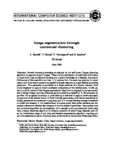
In modern oncology for detecting tumours, photodynamic diagnostics (PDD) is applied. This type of diagnostics is based on the phenomenon of different fluorescence of cancer tissues (reddish light visible in the central part of the colour version of Fig. 1) and healthy tissues (greenish light visible in the upper part of the colour version of Fig.1) in laser blue light. A special fluorescent video endoscope, used in PDD, is the source of colour images of examined tissues (Fig. 1). For the experiment, a representative set of eight colour endoscopic images (I1 , . . . , I8 ) was chosen. These images had the same spatial resolution (768 × 576 pixels) and 24-bit colour depth. During tests the following parameters of clustering techniques were used: colour space, RGB, the number of clusters k = 5, 6 and 7 (selected experimentally), the number of iterations, 15, p = 2.5 (KHM) and initialization method, SD. The value of parameter p is chosen experimentally to process this type of images. After image segmentation by clustering (KM, KHM) we evaluated segmentation results with the help of the above VM (I) and Q(I) indices. Tables 1–3 contain the experimental data.

(a)

The analysis of data in Tables 1–3 leads to the conclusion that the KHM method segments better than KM. We can observe that the VM (I) values are smaller in the case of the KHM technique i.e., an image is better clustered by the KHM method. The second index Q(I) in 23 cases out of 24 is considerably smaller for images segmented by theKHM. Clustering is an iterative process, i.e., it often needs a large number of iterations to reach the stop condition. During each iteration many computations were performed on each pixel, which considerably extended the computation time. Additionally, this time, the spatial resolution of the image and the number of clusters grew up together.

(b)

(c)

Fig. 1. Example of endoscopic image segmentation (grey level version): original image I4 (a), KM based segmentation (b), KHM based segmentation (c).

The computation time can be shortened by using multithread programming and multi-core CPUs. The programmer can create many threads within one process. Every thread disposes its area in operating memory and can get access to the process variables. We proposed a parallelization of computations by uniformly splitting images into sub-images. The number of sub-images is equal to the number of CPU cores. For example, in the case of a Quad Core processor the main thread splits in each iteration the image matrix into four parts and creates four additional computational threads. The operating system, balancing the load in CPU cores, assigns one computational thread to each core. The main thread checks the stopping condition after finishing computations in individual cores and aggregates the results. If the stopping condition is not reached, then the next iteration is executed. After reaching the stopping condition, the main thread writes down the output image and presents the obtained results. More information about parallelization results is given by Frackiewicz ˛ and Palus (2009b).

M. Frackiewicz ˛ and H. Palus

208

6. Postprocessing Clustering techniques used for image segmentation have to be completed by the procedures of region labelling and postprocessing, e.g., adding small regions to the most similar large neighbour regions. One of the most effective methods of postprocessing is to remove the small regions from the image and to merge them into the neighbouring region with the most similar colour. It is not a difficult task, because after region labelling we have a list of regions that can be sorted according to their area. The threshold value of the area of a small region depends on the image. In one image the same threshold allows removing unnecessary artefacts, e.g., highlights or noise and in the other image it removes necessary details. After merging a small region, the mean colour of the new region is computed and the labels of pixels of the small region are changed. As result of such postprocessing, the number of regions in the segmented image significantly decreases. Endoscopic images are very noisy and therefore after segmentation we can observe many small regions in the image. Applying postprocessing with definition of the small region as smaller than 100 pixels decreases the number of regions (Table 4) and improves the value of Q(I) (Table 5). After postprocessing, the KHM technique still preserves its superiority over the KM one.

7. Conclusions In comparison with the classic KM technique, KHM leads to better results of endoscopic image segmentation. Postprocessing based on small region removal improves the results of segmentation. As directions of further research, we can propose the following ideas: considering pixel neighbourhood information in the segmentation process by the KHM method, comparing KHM results with those of other techniques, e.g., region-based segmentation techniques and with those of manual segmentation by a doctor.

Acknowledgment The second author’s participation in this work has been partially supported by the Polish Ministry of Science and Higher Education under Grant No. R13 046 02. The first version of this paper was presented during the 15th National Conference on Application of Mathematics to Biology and Medicine held in Szczyrk, Poland, in 2009 and published in a shortened form in the conference proceedings.

References Bezdek, J.C. (1981). Pattern Recognition with Fuzzy Objective Function Algorithms, Kluwer Academic Publishers, Norwell, MA. Borsotti, M., Campadelli, P. and Schettini, R. (1998). Quantitative evaluation of color image segmentation results, Pattern Recognition Letters 19(8): 741–747. Cheng, H., Jiang, X., Sun, Y. and Wang, J. (2001). Color image segmentation: Advances and prospects, Pattern Recognition 34(12): 2259–2281. Frackiewicz, ˛ M. and Palus, H. (2009a). Initialization methods for clustering in colour image quantization, Proceedings of the 7th Conference on Computer Methods and Systems (CMS’09), Cracow, Poland, pp. 469–472. Frackiewicz, ˛ M. and Palus, H. (2009b). KM and KHM clustering techniques: Computing acceleration by multithread programming, Proceedings of the 7th Conference on Computer Methods and Systems (CMS’09), Cracow, Poland, pp. 333–338. Hamerly, G.J. (2003). Learning Structure and Concepts in Data through Data Clustering, Ph.D. thesis, University of California, San Diego, CA. Linde, Y., Buzo, A. and Gray, R. (1980). An algorithm for vector quantizer design, IEEE Transactions on Communications 28(1): 84–95. Lloyd, S. (1982). Least squares quantization in PCM, IEEE Transactions on Information Theory 28(2): 129–137. MacQuenn, J. (1967). Some methods for classification and analysis of multivariate observations, Proceedings of the 5th Berkeley Symposium on Mathematics, Statistics, and Probabilities, Berkeley CA, USA, pp. 281–297. Palus, H. (2006). Color image segmentation: Selected techniques, in R. Lukac and K. Plataniotis (Eds.), Color Image Processing: Methods and Applications, CRC Press, Boca Raton, FL, pp. 103–108. Zhang, B. (2000). Generalized k-harmonic means—Boosting in unsupervised learning, Technical Report TR HPL-2000137, Hewlett Packard Labs, Palo Alto, CA. Zhang, B., Hsu, M. and Dayal, U. (1999). K-harmonic means— Data clustering algorithm, Technical Report TR HPL1999-124, Hewlett Packard Labs, Palo Alto, CA. Mariusz Frackiewicz ˛ received his M.Sc. degree in automatic control and robotics from the Silesian University of Technology in Gliwice, Poland, in 2006. At present he is a Ph.D. student and his main research interests cover colour image processing. In addition to that, he is also interested in computer programming, computer architectures and modern computer networks.

KHM clustering technique as a segmentation method for endoscopic colour images Henryk Palus received the M.Sc. degree in industrial electronics from the Moscow Power Engineering Institute (MEI) in 1981, and Ph.D. and D.Sc. (habilitation) degrees in automatic control and robotics from the Silesian University of Technology in Gliwice, Poland, in 1990 and 2007, respectively, where he was promoted to the rank of a professor in 2009. His research interest is focused on different problems of colour image acquisition, representation and processing. In 2002–2006 he co-organized international conferences on computer vision and graphics (ICCVG) and edited the proceedings. He is a member of the advisory board and a reviewer of Machine Graphics and Vision, a charter-member of the Polish Association of Image Processing (TPO, IAPR member), and a member of the Commission of Metrology of the Polish Academy of Sciences, Katowice Branch. He is an author or coauthor of more than 80 papers in international and Polish journals as well as conference proceedings.

Received: 8 February 2010 Revised: 2 May 2010

209