estimation of the plant while estimating a function approximation of the difference between the ... intercept point or an angle or a point used to follow ... defined for successful intercept. .... The state estimate Ë x k|k is dependent on two factors:.
KINEMATIC PREDICTION FOR INTERCEPT USING A NEURAL KALMAN FILTER Stephen C. Stubberud*, Kathleen A. Kramer** *The Boeing Company, Anaheim, CA 92805 ** Department of Engineering, University of San Diego, San Diego, CA, 92110
Abstract: The neural extended Kalman filter is a technique that learns unmodelled dynamics while performing state estimation. This coupled system performs the state estimation of the plant while estimating a function approximation of the difference between the system model and the dynamics of the true plant. At each sample step, this approximation is added to the existing model improving the state estimate. This neural estimator is applied to a two-dimensional intercept problem as a target tracker providing the control reference signal. Comparisons between different prediction times used in the control are provided for both the neural tracker and a baseline tracker. Copyright © 2005 IFAC Keywords: Neural networks, Kalman filters, Target tracking, Data fusion, Control accuracy.
1. INTRODUCTION The target intercept problem is an important component of robotics, space systems, and missile defence. This guidance and control problem has been analyzed for a number of years (Zarchan, 2002). The reference signal, whether a predicted intercept point or an angle or a point used to follow the target while in motion, must be accurately defined for successful intercept. These signals are either provided a priori using a model of the trajectory or by in-flight position coordinates. Usually, the actual motion model of the target is unknown, and the interceptor must rely upon target tracks provided by off-board sensors. These offboard tracks, in order to reduce the effects of noise on the measurements, rely upon a target motion model. A manoeuvre that is not properly compensated for in the tracking system can cause a lag in tracking performance or corruption by noise. In the control loop for an interceptor, as depicted in Figure 1, the reference input is a predicted state estimate from the tracker. The reference signal is either a long term prediction or prognostication that
Predicted Target Location
+ _
K
G(z)
Interceptor
Position/Velocity
Fig. 1: The interceptor control is based on an estimate of the desired reference input. is used to enable the interceptor to meet the target at a given point or a short term prediction used to enable the interceptor to follow and strike the target. This predicted estimate is the output of the target tracker processed through its motion model. Better tracker estimates of the state of the target (position and velocity) and a more accurate model of the target motion increase the probability of intercepting the target. To compensate for the lag in the tracking behaviour of a manoeuvring target, adaptive and approximating estimation routines have been developed (Kirubarajan and Bar-Shalom, 2003) and (Wang and Varshney, 1993). Another such approach is the neural extended Kalman filter (NEKF). In (Stubberud and Kramer, 2004), the application of the
NEKF to the target tracking problem for target intercept using a long term predictive intercept point was introduced. The NEKF is able to track accurately through manoeuvres without a priori knowledge of the manoeuvre motion model. The NEKF provides both an improved state estimate and an improved motion model. The NEKF, as defined in (Stubberud, et al., 1998) and (Stubberud, et al., 1995), is a Kalman filter that uses a neural network to improve the state-coupling function used in the prediction step of the state estimate (target track). The neural network trains online to learn the difference between the dynamics of the existing system and the model used by the Kalman filter. The NEKF is both the state estimator and the neural network trainer. Both components use the same measurement information. The improved motion model that NEKF provides increases the accuracy of the predicted location of the target. The model of the motion used by the NEKF is a sum between an initial model and the neural network. While the model of the neural network is continually adapting based on the data, a prediction using the weights at a given time can be made to an arbitrary time into the future. While the accuracy of this prediction deteriorates the further in the future one predicts, the average performance should be better than that of the non-corrected model. The goal of this effort is to show the benefit of short-term prediction in the target tracking used as the reference signal for the control loop of the interceptor. In Section 2, the theoretical development of the NEKF is summarized. The basic control approach to the intercept problem with the NEKF implemented is discussed in Section 3. In Section 4, the example problem is described. The results of the NEKF are compared against a standard Kalman filter in Section 5 for predictions of 1, 2, and 5 seconds. 2. THE NEURAL-EXTENDED KALMAN FILTER The neural extended Kalman filter is a coupled system of a standard EKF that provides state estimates and an EKF neural network training parameter as developed in (Singhal and Wu, 1989). The standard EKF equations are given as
K k = Pk |k −1
∂h ( xˆ k |k −1 , u k ) ∂xˆ k |k −1
×
∂xˆ k |k −1
) (1b)
∂h ( xˆ k |k −1 , u k ) Pk |k −1 Pk |k = I − K k ∂xˆ k |k −1 (1c)
(
xˆ k +1| k = f xˆ k | k , u k
)
(1d)
(
∂f xˆ k | k , u k Pk +1| k = ∂xˆ k | k
(
∂f xˆ k | k , u k ∂xˆ k | k
)T
)
P × k |k
(1e)
+ Qk
The state estimate xˆ k| k is dependent on two factors:
the measurements, z k , and the process model, f (⋅) . The quality of the process model has a significant impact on the state estimate. The process model is a matrix function that estimates the dynamics of the target
f true = f (⋅) + ε The error in the model can be estimated arbitrarily close using a function approximation scheme. As discussed in (Owen and Stubberud, 2003), this is a result of the Stone-Weiestrauss Theorem. A neural network fits the criteria of this theorem if it uses a multi-layer perceptron. In (Stubberud, et al., 1993), a neural network training algorithm using the EKF paradigm was coupled to an EKF performing state estimations. This implementation is detailed in Figure 2. The new state includes the target states and the weights of the neural network. zk
+ _
Σ
zk − zˆk
xˆ u
Σ
K
xˆ p h(xˆ p )
xˆ p
Σ
ˆ w f (xˆ u )
ˆ) NN (xˆ u , w
T
×
∂h ( xˆ k |k −1 , u k ) Pk|k −1 ∂xˆ k |k −1 ∂h ( xˆ k |k −1 , u k )
(
xˆ k |k = xˆ k |k −1 + K k z k − h ( xˆ k |k −1 , u k )
+ Rk
(1a) −1
Fig. 2: Implementation of the NEKF – A neural network training algorithm is coupled to an EKF performing state estimation. The same residuals used to update the state estimator also train the weights to provide a function that, when added to the original mathematical model
f true = f (⋅) + NN (⋅) + δ δ < ε, provides an improved dynamic model for the prediction step (Eqs. (1d) and (1e)). The coupled equations of the NEKF are defined as
)
(
−1 K k = Pk | k −1H Tk H k Pk|k −1H Tk + R k (2a)
better than those provided by Eqs. (1d) and (1e). The motion model of the target is provided by the initial NEKF motion model with the neural network added in
xˆ k + n | k = f predicted (xˆ k | k , n) ˆ k | k , n) = f (xˆ k | k , n) + NN (xˆ k | k , w where the weights are held constant. 3. INTERCEPT CONTROL SYSTEM
xˆ k |k
xˆ k |k xˆ k |k −1 = = + ˆ k |k w ˆ k |k −1 w
(
K k z k − h ( xˆ k |k −1 , u k )
(2b)
)
Pk | k = (I − K k H k )Pk | k −1
(2c)
xˆ k +1| k w = ˆ + 1 | k k ˆ k |k f xˆ k | k , u k + NN xˆ k | k , u k , w ˆ k |k w
(
)
(
The discrete-time model of the interceptor is defined as
)
(
ˆ k |k , u k ∂NN xˆ k |k , w Pk +1|k = F + ∂xˆ k |k
(
ˆ k|k , u k ∂NN xˆ k |k , w F + ∂xˆ k |k
)T
)
(2d)
P × k |k
+ Qk (2e)
ˆ is the augmented state vector of Eq. (2b) where x k |k and
F 0 F= , 0 Iw
(3)
where the Jacobian of our a priori model F is defined by
Fij =
∂ fˆk (•)i ∂x j 0w
0 dt 2 2 1 dt 0 0 0 1 0 0 0 dt u x + x k +1 = k 2 0 0 1 dt k 0 dt 2 dt 0 0 0 0 1 1 0 0 0 yk = xk 0 0 1 0 where the state is defined as the discretized version of target kinematics of position and velocity for a sample rate of dt
x x& x= y y& For both coordinates, x and y, there are two controllers in series
x = xˆ k|k
G x ( z ) = G y ( z ) = G1G2
and
∂h ( x k |k −1 , u k ) H= ∂xˆ k |k −1
The intercept control problem employed uses the standard feedback control approach seen in Figure 1. The controller used is a double-lead controller. Sample rates of 1.0, 2.0, and 5.0 seconds were used. The reference input was a predicted location of the target based upon the sample time. The reference signal was the predicted location of the target provided by the target tracking system.
where (4)
The augmented state vector estimates simultaneously the track estimates and the weights of the neural network. The weights of the neural network are considered parameters of a function. These weights are adjusted by the residual to correct errors in the prediction. The weights change the model used in Eqs. (2d) and (2e). Thus, the prediction estimates are
G1 =
z − 0.3 z + 0.4
G2 =
z − 0.8 z − 0.2
with a gain, K, chosen as 1.0, 0.33, and 0.05 for a sample rate of 1.0, 2.0, and 5.0 seconds, respectively.. These were chosen to ensure stability of the interceptor.
4. EXAMPLE PROBLEM
5. RESULTS OF THE KALMAN FILTER AND THE NEKF
For our test case, a target with a ballistic trajectory was created. The continuous time model of the system was defined as
0 0 x& (t ) = 0 0
1 0 0 0
0 0 0 0
0 1 0 0 x(t ) + 0 1 0 0
0 1 0 0
0 0 u(t ) 0 1 (5)
x&
1 0 0 0 H= 0 0 1 0
(6)
The measurement covariance was defined as
R = 2500 ⋅ I 2×2
(7)
based on the noise added to the measurements.
The state x was defined as
[x
The target was tracked using both a Kalman filter and the NEKF. The measurement-coupling equation for the state estimates was defined for position-only measurements
y
y& ]
T
which represents the x, y coordinate of the target and the associated velocities. The input u was defined as
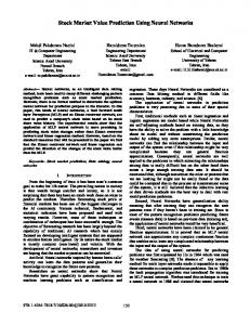
rot _ earth ax f − g where rot _ earth indicates the rotation of the earth for a given time step, a x defines any x-direction acceleration provided by the target, f − g indicates the vertical acceleration of the target with the effects of gravity. For our test case, the sampling rate to discretize the system was set to 1 second. The rotation of the earth was set to (20000/(24⋅3600)) m/s. The horizontal acceleration was defined as 40 m/s2 for the duration of the trajectory. The applied vertical acceleration was set at a value of 12 m/s2 and lasted for 60 seconds. Figure 3 shows the resulting test case trajectory.
Fig. 3: Example target trajectory used as test case.
The process noise covariance was defined as the integrated white noise model
dt 3 3 dt 2 2 0 0 2 dt 2 dt 0 0 (8) Q = 0.01 0 0 dt 3 3 dt 2 2 0 dt 2 2 dt 0 The initial model of the NEKF is given as the straight-line motion model of Eq. (5) sampled at 1.0 second intervals. The input-coupling matrix was set to zero in that the actual inputs are not known. For the NEKF, a single-layer neural network with four hidden nodes that applied a sigmoid function
1 − e− α 1 + e− α was used. The process noise was 1.0 on the input weights and 0.05 for the output weights. Target track predictions of 1.0, 2.0, and 5.0 seconds ahead were used to create the reference signal in the control system. The interceptor was launched at 34 seconds into the 106 second flight of the target. 100 Monte Carlo runs were performed for each prediction time using the noise statistics described above. The average miss distances between the NEKF predictions and the true path were measured. These are shown in Figure 4. The one step prediction is shown as the solid line. The dashed-dotted line depicts the two time-step prediction while the dashed line indicates the results of a five time-step prediction. This notation is used also used in Figures 5, 6, and 7. In Figure 5, the results runs that were repeated using the Kalman filter are shown. As was expected, the shorter prediction time, the better its accuracy was found to be. The prediction values from the two tracking approaches were then used as the reference signal of the interceptor control loop. The results for the interceptor for each prediction time are shown in
Figures 6 for the NEKF results and Figure 7 for the Kalman filter results.
14000
From these results, it is clearly seen that the NEKF provides superior results to the Kalman filter when used as the tracking system that provides the reference signal to the control system.
6000
4000
0 30
40
50
60
70 step
80
90
100
110
Fig. 7: Interceptor Results Using Kalman Filter Prediction.
1-step predict 2-step predict 5-step predict
Table 1. Mean Miss Distance Between Interceptor and Target
1600 1400 1200
distance (m)
8000
2000
2000 1800
10000 distance (m)
Table 1 details the mean miss distance of the interceptor for both tracking approaches. Table 2 details the standard deviation of the miss distance of the interceptor for both tracking approaches. The statistics were taken beginning from 16 seconds into the flight of the interceptor, so as to remove the initial launch distances.
1-step predict 2-step predict 5-step predict
12000
Prediction NEKF Kalman Filter
1000 800 600
1.0 s 197.6 3084
2.0 s 446 3311
5.0 s 2693 4114
400 200 0
0
20
40
60 step
80
100
120
Fig. 4: Average Miss Distance Between Path and Prediction Using NEKF.
Prediction NEKF Kalman Filter
7000 1-step predict 2-step predict 5-step predict
6000
distance (m)
5000
1.0 s 37.7 1464
2.0 s 139.2 1490
5.0 s 626.9 1577
6. CONCLUSIONS
4000
3000
2000
1000
0
0
20
40
60 step
80
100
120
Fig. 5: Average Miss Distance Between Path and Prediction Using the Kalman Filter. 1-step predict 2-step predict 5-step predict
16000
In this paper, the use of a neural extended Kalman filter to provide a continual state estimate and to, in turn, use these results for interception of the target was introduced. As in its use for a closed-loop control system, the NEKF was shown to have the capability to improve the state estimates in the presence of modelling errors. The goal of this research is to provide an improved ability to intercept the target. From these results, paths of continued research present themselves. Incorporation of predictive location control into the system could significantly improve ability to intercept. One step is to incorporate noise into the measurements. In past work, the NEKF has shown greater performance with noisy signals and greater variation in the training dynamics (Stubberud and Owen, 2000), (Stubberud and Owen, 1999), and (Stubberud and Owen, 1996). Another path towards improving intercept ability is that the neural network training parameters need to be investigated further to improve performance.
18000
14000 12000 distance (m)
Table 2. Standard Deviation of Miss Distance Between Interceptor and Target
10000 8000 6000 4000 2000 0 30
40
50
60
70 step
80
90
100
110
Fig. 6: Interceptor Results Using NEKF Prediction.
The current example uses a simplified interceptor model and controller. As this research continues, the interceptor model and associated control law will be
investigated further. Control laws to be considered include predictive control and proportional navigation. REFERENCES Kirubarajan, T and Y. Bar-Shalom, “Tracking Evasive Move-Stop-Move Targets With A GMTI Radar Using A VS-IMM Estimator,” IEEE Transactions on Aerospace and Electronic Systems, Vol. 39 , No. 3, pp. 1098 – 1103, July 2003. Owen, M.W. and A.R. Stubberud, “NEKF IMM Tracking Algorithm,” Proceedings of SPIE: Signal and Data Processing of Small targets 2003, Vol. 5204, Oliver Drummond (ed.), San Diego, California, August, 2003. Singhal, S, and L. Wu, “Training Multilayer Perceptrons with the Extended Kalman Algorithm,” Chapter, Advances in Neural Processing Systems I, D.S. Touretsky (ed.), Morgan Kaufmann, pp. 133-140, 1989. Stubberud, S.C. and K .A. Kramer, “A 2-D Intercept Problem Using a Neural Extended Kalman Filter and Controller Modification,” Proceedings of the International Conference on Computing, Communications and Control Technologies, Vol. 4, pp. 228-233, Austin, TX, August, 2004. Stubberud, S.C., R.N. Lobbia, and M. Owen, “An Adaptive Extended Kalman Filter Using Artificial Neural Networks,” Proceedings of the 34th IEEE Conference on Decision and Control, New Orleans, pp. 1852-1856, Louisiana, December, 1995. Stubberud, S.C., R.N. Lobbia, and M. Owen, “An Adaptive Extended Kalman Filter Using Artificial Neural Networks,” The International Journal on Smart System Design, Vol. 1, pp. 207-221, 1998. Stubberud, S. and M. Owen, “Controller Modification Using Improved Models Of The Neural Extended Kalman Filter,” Proceedings of the 14th International Conference on Systems Engineering, Coventry, UK, pp. 519-523, September, 2000. Stubberud, S. and M. Owen, “An On-line Control Law Adaptation Technique Using Neural Networks,” Proceedings of the 13th International Conference on Systems Engineering, Las Vegas, NV, August, 1999. Stubberud, S.C. and M. Owen, “Artificial Neural Network Feedback Loop,” Proceedings of the 11th International Symposium on Intelligent Control, pp. 514-519, Dearborn, Michigan, September, 1996. Stubberud, S.C., V. Samant, and J. Saib, “Neural Network Technique for an Adaptive Estimator for Dynamic Systems,” Proceedings of the Ninth International Conference on Systems Engineering, Las Vegas, NV, pp. 230-234, July 15-17, 1993.
Wang, J.C. and P.K. Varshney, “A Tracking Algorithm For Maneuvering Targets,” IEEE Transactions on Aerospace and Electronic Systems, Vol. 29, No. 3, pp. 910-925, July, 1993. Zarchan, P., Tactical and Strategic Missile Guidance, Fourth Edition, American Institute of Aeronautics and Astronautics, Washington, D.C., 2002.