Knowledge extraction based on wavelets and DNN for classification of

Knowledge extraction based on wavelets and DNN for classification of physiological signals: Arousals case E Macias, A Morell, J Serrano, JL Vicario Wireless Information Networking, Univeritat Aut`onoma de Barcelona, Spain Abstract With a large amount of data collected from studies of sleep quality and based on the physiological signals (PS) that are collected, it is possible to use mechanisms that intelligently detect sleep disorders such as arousals (ARS). In this detection, the triggers can be present in any of the PS or can occur from their combinations. Thus, with the characterization of the PS and with a considerable number of examples, it is possible to generate a model that recognizes ARS zones in new samples. In this way, by segmenting the signals and decomposing them into variable frequency bands, thanks to the application of discrete wavelet transform (DWT), it is possible to characterize the contributions of each PS in time and frequency. The features that are extracted give information about the contributions in frequency and time of each PS. Then these characteristics feed a neural network model that iteratively learns the best non-linear function that approximates the input to its corresponding label. Once the methodology was tested, with less than 3% of the training data, it was possible to reach an Area Under Precision-Recall Curve (AUPRC) of 0.261.

1.

Introduction

In medicine with the increase of information that Big Data era has brought, and thanks to the knowledge extraction tools, it is possible to capture relevant information on large amounts of data efficiently. Thus, in the context of the study of sleep disorders, with different physiological signals (PS) collected by sensor networks through Polysomnography studies, it is possible to obtain information of approximately 4-7 hours, and based on this, use mechanisms that facilitate their analysis and help to find related pathologies. On the other hand, regarding sleep activity, its function is to save energy to generate a physiological stabilization. In a normal health condition a person can pass through several cycles, each lasting 90-110 minutes [1]. These are composed by two primary states known as rapid eye movement (REM) and non-rapid eye movement (non-REM).

The sleep cycle starts with the non-REM state, which has 4 sub-phases through which a person begins with drowsiness and ends at the beginning of deep sleep. During this state, several neuronal systems are activated, while others are deactivated so that the body enters a phase of deep sleep [2]. From phase 4, it is passed to the REM state where, paradoxically, the nervous system goes into alert mode while the muscles are in the state of maximum relaxation. However, different sleep disorders do not allow recovery to be carried out, among them, according to the International Classification of Sleep Disorders (ICSD) [3], those where there are problems of drowsiness, disorders associated with medical complications, and those where occur ARS. The last one is due to sudden changes in the activity of brain waves. It can also be interpreted as the change in sleep states, from a non-REM state to REM or REM state when the subject is awake. Thus, in this work is proposed the detection of ARS zones, in the context of ”You Snooze, You Win: the PhysioNet/Computing in Cardiology Challenge 2018” [4], based on the segmentation, extraction of features on discrete wavelet transform (DWT), applied to PS, and its subsequent classification, using an artificial neural network (ANN) as a classification mechanism.

2.

Materials and methods

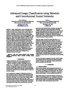
For this challenge, there were 1893 records, with 13 PS, see Fig 1, which included electrocardiograms (ECG), oxygen saturation (SaO2), respiratory flow and various derivations of electroencephalography (EEG) and electromyography (EOM) [4]. The goal of the Challenge was to classify ARS zones present in the PS. The following are the methods to carry out the extraction of features and their subsequent classification.

2.1.

Segmentation

Each record contains more than 4 million samples, labeled with three possible classes, ’-1’, ’0’ and ’1’ referring to unimportant, non-ARS and ARS class, respectively. Only the non-ARS and ARS classes are used for clas-

d3

an

fs/2^n Segm 1

fs/16

d2

fs/8

d1

fs/2

fs/4

Segm 2

Figure 1. zoom with a window of 10000 samples over the 13 PS

Figure 2. Spectrum distribution according to number of levels, n

sification. Initially, the PSs are segmented with a window of length N, so a record with L samples will contain M = LmodN segments, that will serve either to train a model or to test it on new samples, as is the case of the test data. For training, when segmenting the PS, each sample of the segment carries its label. A single label is defined for the entire segment according to the majority found in the label window. Similarly, a pair of rules are defined to deal with the start and end of the files, according to their distributions, as follows: • As indicated above, with the mod operation, the remaining samples are taken directly to class ’0’ due to the distribution and the assumption that the patient finishes the analysis awake. • First 100,000 samples of each record are discarded due they do not present ARSs. For this work, segments of 12.5 seconds of duration (2500 samples) were taken. On the other hand, the data of the non-ARS class represent 75-85% of the total of a sample, while the ARS are between 5-11%. In order to have balanced data, the same number of segments of the non-ARS class, selected randomly, and ARS segments are taken.

quency bands that describe known events, such as sleep states based on EEG [6], characterization of ECG [7], extraction of electromyography information [8], among others.

2.2.

Analysis using discrete wavelet transform

The Wavelet transform (WT) is a spectral estimation technique which allows decomposing a signal in linear combinations, dilating and moving a function called a mother wavelet, see Eq 1, where a and b are the scaling and translation parameters, respectively. By varying these parameters and moving the mother wavelet, its correlation with the signal segments is calculated, as indicated by Eq 2. The usefulness of the wavelets lies in time-frequency location, a feature that can not be reached with the Fourier transform or the STFT[5]. In this way, the WT offers an outstanding frequency resolution analysing long time windows and the detection of abrupt changes in time when analyzing high frequencies [5]. The application of this type of segmentation in PS turns out to be very useful, since it allows to extract relevant information about fre-

1 t−b ψa,b (t) = √ ψ( ) a a

Ws f (x) = f (x)∗Ψs (x) =

1 s

Z

(1)

+∞

f (t)Ψ( −∞

x−t )dt (2) s

On the other hand, each wavelet acts as a filter, extracting the time evolution of the components of the original signal contained in the frequency bands associated with those determined in the wavelets, Fig 2 shows the distribution of bands that would correspond to each wavelet. These bands are defined based on quadrature mirror filters [9], where a signal is divided into two bands resulting from the application of a low pass filter (LPF) and a high pass filter (HPF). Then, the band corresponding to low frequencies is divided sequentially generating levels, in such a way that in each of them the HPF preserves the details of the signal and the LPF represents the trend or coarse approximation of the signal [9]. Fig 3 presents an outline of this.

g[n] g[n]

h[n] h[n]

2

2

h[n]

2

A3

2

2

X[n]

g[n]

2

D3

D2

D1

Figure 3. subband decomposition, h[n] is the HPF and g[n] LPF, after each filter the signal is decimated For this work the DWT Daubechies of order 6 was used, decomposing the PS in 7 levels and whose sub-bands are shown in Table 1. From this decomposition, only the coefficients of the details D2-D7 were used due there are no relevant events in the 50-100Hz band.

2.3.

Feature extraction

Once the PS are segmented, and these segments have decomposed into 6 details, next is the feature extraction. As in [10], in order to know the time and frequency contributions in each band, the following features are calculated on the coefficients of each sub-band: • Mean of the absolute values of the wavelets coefficients. • Average power of the wavelet coefficients. • Standard deviation of the coefficients. • Ratio of the absolute mean values of adjacent sub-bands. Thanks to this extraction of features in each PS, it was possible to transform 32500 samples, produced from the 13 PS, to 312, these were the ones that fed the model for training.

Hidden layer 1

Inputs

U11

x1

U12

x2

U13

Artificial neural networks

The goal of artificial neural networks (ANN) is given a set of input examples, x = [x1 , ..., xn ]T and their labels y = [y 1 , ..., y l ], for the case of classification, learn the best non-linear function that presents the smallest error between the classified input and its output. Structurally, an artificial neural network (ANN) has layers, neurons, and their interconnections, as shown in Fig 4. Each layer is formed of interconnected units called neurons. There are three types of layers, the input, where the original data is entered and is where the patterns are presented, this is connected to one or more (deep neural network) hidden layers and in the end these are connected to the output layer that is responsible for transforming its input to the desired output format. The connections carry a weight that is multiplied by the input of the layer and then it is passed through a non-linear P function. This generates an activation function a = f ( i xi ∗ wi + b) (see Fig 5) which maps the input to a range of values. The learning process of the network is carried out through the iterative updating of the weights, starting with random assigned values, then minimizing the error through a cost function, which in our case will be done with crossentropy (see Eq 3).

Table 1. Frequency band distribution Descomposed signal Frequency band (Hz) D1 100-200 D2 50-100 D3 25-50 D4 12.5-25 D5 6.2-12.5 D6 3.1-6.2 D7 1.6-3.1 A7 0-1.6

U21

Wji

Output

U22

U14

xi

y1

U2k

Wkj

U1j

yk

U2l

xn U1m

Figure 4. Artificial neural network with on hidden layer b

2.4.

Hidden layer 2

Activation function: a

Weigths

x1 W1

x2

xn

Output W2

Wn

Inputs

Figure 5. Single unit in a layer

m

1 X (i) J(Θ) = − y log(f (x(i) )) m i=1 + (1 − y (i) ) log(1 − f (x(i) )) +

λ 2m

(3)

sl sX L−1 l +1 XX

(Θlj,i )2

l=1 i=1 j=1

where L is the number of layers of the ANN, sl the number of units in the l-th layer, k the output units, λ > 0 a regularization parameter and θ contains all the weigths of the ANN. Once the output is obtained, and it is compared with the desired one, based on the value of the cost function, the weights of the network are updated based on the backpropagation algorithm [2]. To carry out the classification we used an ANN with 2 hidden layers, with 200 and 100 neurons respectively, with a learning rate lr = 1e−4 with Adam optimizer and using L2 regularization with β = 1e−2 and a dropout = 0.7, dropping 30% of the connections in each iteration of the training.

2.5.

Metrics

To measure the effectiveness of the model in the classification of the ARS and non-ARS regions, the area under

Acknowledgements

the precision-recall curve was calculated as follow: Arspred Rj = P T otalArs

(4)

Arspred (5) T otalSamples where Arspred is the number of ARSP samples with predicted probability (j/1000) or greater, T otalArs the toP tal number of ARS samples and T otalSamples the total number of samples with predicted probability (j/1000) or greater. And the final score is measured thought the gross AUPRC. X AU P RC = Pj (Rj − Rj−1 ) (6) Pj = P

j

This metric gives information about the relationship between sensitivity and positive predicted value and takes values is in the range of 0 to 1.

3.

Results

This work was done with Python on a MacBook Pro, 2.4 Ghz Intel Core i5, 8 GB 1333 MHz DDR3, Intel HD Grafics 3000 512 MB. Taking segments of 2500 samples for each PS, extracting the information of 6 details in the bands of interest on each PS, through the 4 characteristics, and trained with balanced segments, 44680, of 30 records, it was possible to obtain an AU P RC = 0.261 on the rest of the data (968) of the training set. The highest score for the challenge was 0.6 applying deep learning algorithms. On the other hand, to reach the capacity of the model, it was enough to train with 3% of the available data, taking into account the imbalance of the samples and the computational limitation.

4.

Discussion

As evidenced in the Challenge, the detection of arousal zones is not a trivial problem. Then, it is necessary to integrate different mechanisms for the representation and extraction of knowledge from the PS. In this way, in this work it was possible to design a simple learning model, which provided good performance concerning computational resources, through the synthesis of information, transforming segments of 32500 to its representation in 312 samples that correspond to the contributions of each segment in several frequency bands. It is also important to consider data augmentation techniques where artificial samples can be generated, in order to increase the quantity in unbalanced classes and thus use more segments of the class with larger samples, and be able to feed the model, in a balanced way, with more samples.

This work is supported by the Spanish Government under Project TEC2017-84321-C4-4-R co-funded with European Union ERDF funds and also by the Catalan Government under Project 2017 SGR 1670.

References [1]

Slopen N, Lewis TT, Williams DR. Discrimination and sleep: A systematic review. Sleep Medicine 2016;18:88– 95. ISSN 18785506. [2] Ebrahimi F, Mikaeili M, Estrada E, Nazeran H. Automatic sleep stage classification based on EEG signals by using neural networks and wavelet packet coefficients. 2008 30th Annual International Conference of the IEEE Engineering in Medicine and Biology Society 2008;1151–1154. ISSN 1557-170X. [3] Sateia MJ. International classification of sleep disordersthird edition highlights and modifications. Chest 2014; 146(5):1387–1394. ISSN 19313543. [4] Mohammad M Ghassemi, Benjamin E Moody, Li-wei H Lehman, Christopher Song, Qiao Li, Haoqi Sun, Roger G. Mark, M Brandon Westover GDC. You Snooze, You Win: the PhysioNet/Computing in Cardiology Challenge 2018, 2018. [5] Shoeb A, Clifford G. Wavelets ; Multiscale Activity in Physiological Signals Short-Time Fourier Transform. Biomedical Signal and Image Processing 2006;1–29. [6] Eckert DJ, Younes MK. Arousal from sleep: implications for obstructive sleep apnea pathogenesis and treatment. Journal of Applied Physiology feb 2014;116(3):302– 313. ISSN 8750-7587. [7] Subasi A. EEG signal classification using wavelet feature extraction and a mixture of expert model. Expert Systems with Applications 2007;32(4):1084–1093. ISSN 09574174. [8] Jain V, Crochiere R. Quadrature mirror filter design in the time domain. IEEE Transactions on Acoustics Speech and Signal Processing 1984;32(2). ISSN 0096-3518. [9] Li C, Zheng C, Tai C. Detection of ECG characteristic points using wavelet transforms. IEEE Trans Biomed Eng 1995;42(Bmei):21–28. ISSN 00189294. [10] Kumar DK, Pah ND, Bradley A. Wavelet analysis of surface electromyography to determine muscle fatigue. IEEE Trans Neural Syst Rehabil Eng 2003;11(4):400–406.