DATA COMPRESSION in IMAGE PROCESSING using SVD. Goals. The goal of
this lab is to demonstrate how the SVD can be used to remove redundancies in ...
Lab # 3 - ACS I DATA COMPRESSION in IMAGE PROCESSING using SVD
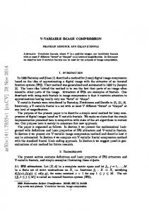
Goals. The goal of this lab is to demonstrate how the SVD can be used to remove redundancies in data; in this example we will be compressing image data. We will see that for a matrix of rank r, the SVD can give a rank p < r approximation to a matrix and that this approximation is the one that minimizes the Frobenius norm of the error. Introduction Any image from a digital camera, scanner or in a computer is a digital image. The “real world” color image is digitized by converting the images to numerical data. A pixel is the smallest element of the digital image. For example, a 3 megapixel camera has a grid of 2048 × 1536 = 3,145,828 pixels. Since the size of a digitized image is dimensioned in pixels of say m rows and n columns, it is easy for us to think of the image as an m × n matrix. However, each pixel of a color image has an RGB values (red, green, blue) which is represented by three numbers. The composite of the three RGB values creates the final color for the single pixel. So we can think of each entry in the m × n matrix as having three numerical values stored in that location, i.e., an m × n × 3 matrix. Now suppose we have a digital image taken with a 3 megapixel camera and each color pixel is determined by a 24-bit number (8 bits for intensity of red, blue and green). Then the information we have is roughly 3 × 106 × 24. However, when we print the picture suppose we only use 8-bit colors giving 28 = 256 colors. We are still using 3 million pixels but the information used to describe the image has been reduced to 3 × 106 × 8, i.e., a reduction of one-third. This is an example of image compression. In the figure below we give a grayscale image of the moon’s surface (the figure on the left) along with two different compressed images. Clearly the center image is not acceptable but the compressed image on the right has most of the critical information. We want to investigate using the SVD for doing data compression in image processing.
Understanding the SVD Recall from the notes that the SVD is related to the familiar result that any n × n real symmetric matrix can be made orthogonally similar to a diagonal matrix which gives us the decomposition A = QΛQT where Q is orthogonal and Λ is a diagonal matrix containing the eigenvalues of A.
1
Figure 1: The image on the left is the original image while the other two images represent the results of data compression. The SVD provides an analogous result for a general nonsymmetric, rectangular m × n matrix A. For the general result two different orthogonal matrices are needed for the decomposition. We have that A can be written as A = U ΣV T , where Σ is an m × n diagonal matrix and U, V are orthogonal. Recall from the notes that the SVD of an m × n matrix A can also be viewed as writing A as the sum of rank one matrices. Recall that for any nonzero vectors ~x, ~y the outer product ~x~y T is a rank one matrix since each row of the resulting matrix is a multiple of the other rows. The product of two matrices T can be written in terms of outer products. In particular, the product P ~ TBC of two matrices can be written as the sum of the outer products i bi~ci where ~bi , ~ci denote the ith columns of B and C respectively. Hence if we let ~ui denote the ith column of U and ~vi the ith column of V then writing the decomposition A = U ΣV T as the sum of outer products we get (1)
A = ~u1 σ1~v1T + ~u2 σ2~v2T + · · · + ~ur σr ~vrT =
r X
σi ~ui~viT .
i=1
where r denotes the rank of A. Thus our expression for A is the sum of rank one matrices. If we truncate this series after p terms, then we have an approximation to A which has rank p. What is amazing, is that it can be shown that this rank p matrix is the best rank p approximation to A measured in the Frobenius norm. Recall that the Frobenius norm is just the matrix analogue of the standard Euclidean length, i.e., 1/2 X A2ij kAkF = i,j
where Aij denotes the (i, j) entry of the matrix A. However, it is NOT an induced matrix norm. 2
We can get a result for the error that is made by approximating a rank r matrix by a rank p approximation. Clearly we have that the error Ep is given by p r X X σi ~ui~viT . σi ~ui~viT = Ep = A − i=p+1
i=1
Due to the orthogonality of U and V we can write kEp k2F =
r X
σi2
i=p+1
and so a relative error measure can be computed from (2)
" Pr
2 i=p+1 σi P r 2 i=1 σi
#1/2
.
Data compression using the SVD How can the SVD help us with our data compression problem? Remember that we can view our digitized image as an array of mn values and we want to find an approximation that captures the most significant features of the data. Recall that the rank of an m × n matrix A tells us the number of linearly independent columns of A; this is essentially a measure of its non-redundancy. If the rank of A is small compared with n, then there is a lot of redundancy in the information. We would expect that an image with large-scale features would possess redundancy in the columns or rows of pixels and so we would expect to be able to represent it with less information. For example, suppose we have the simple case where the rank of A is one; i.e., every column of A is a multiple of a single basis vector, say ~u. Then if the ith column of A is denoted ~ai and ~ai = ki ~u, then A = ~u~k T , i.e., the outer product of the two vectors ~u and ~k where ~k = (k1 , k2 , · · · kn ). If we can represent A by a rank one matrix then all we need to specify are the vectors ~u and ~k; that is m + n entries as opposed to mn entries for the full matrix A. Of all the rank one matrices we want to choose the one which best approximates A in some sense; if we choose the Frobenius norm to measure the error, then the SVD decomposition of A will give us the desired result. Of course in most applications the original matrix A is of higher rank than one so that a rank one approximation would P be very crude. In general we seek p a rank p approximation to A such that kA − i=1 σi ~ui~viT kF is minimized. It is important to remember that the singular values given in Σ are ordered so that they are nonincreasing. Consequently, if the singular values decrease rapidly, then we would expect that fewer terms in the expansion of A in terms of rank one matrices would be needed.
3
Computational Algorithms In this lab, we will treat the software for the SVD as a “black box” and assume that the results are accurate. In this lab, you can either use the LAPACK SVD routine dgesvd or MATLAB commands svd and svds. The LAPACK algorithm can be downloaded from netlib (www.netlib.org). The interested student is referred to Golub and Van Loan’s book for a description of the algorithm used to obtain the SVD. A test image library for use in image compression is maintained by the electrical engineering department at the University of Southern California and the images for this lab were obtained from there. In addtion to the SVD algorithm, we will need routines to generate the image chart (i.e., our matrix) from an image and to generate an image from our approximation. There are various ways to do this. One of the simplest approaches is to use the MATLAB commands imread - reads an image from a graphics file imwrite - writes an image to a graphics file imshow - displays an image Specifics of the image processing commands can be found from Matlab’s technical documentation such as http : //www.mathworks.com/help/toolbox/images/f0 − 18086.html or the online help command. When you use the imread command the output is a matrix in unsigned integer format, i.e., (uint8). You should convert this to double precision (in Matlab double) before writing to a file or using commands such as svds. However, the imshow command wants the uint8 format. You should learn the difference between the Matlab commands svd and svds.
Exercises 1. The purpose of this problem is to make sure you are using the SVD algorithm (either from Matlab or netlib) correctly. First, make sure that you get the SVD of 1 2 3 4 5 6 A= 7 8 9 10 11 12
4
as T .1409 −.8247 −.5456 .0486 25.46 0 0 .5045 .7608 4082 .6912 −.4714 .3439 −.4263 A= 0 1.291 0 .5745 −.05714 .8165 . .5470 −.0278 .2543 .7971 0 0 0 .6445 −.6465 .4082 .7501 .3706 −.3999 −.3743
Next compute a rank 1 approximate to A and determine the error in the Frobenius norm by (i) calculating the difference of A and its approximation and then computing its Frobenius norm and (ii) using the singular values. For this problem just turn in your rank 1 approximation and your error estimates. 2. In this problem we will be using the grayscale image boat.tiff which can be downloaded from my web page. Create an integer matrix chart representing this image. Your image chart should be a 512 × 512 matrix with entries between 0 and 255. View your image (for example with imshow) to make sure you have read it in correctly. a. Write code to create the matrix chart for an image and to do a partial SVD decomposition; you should read in the rank of the approximation you are using as well as the image file name. Use your code to determine and plot the first 150 singular values for the SVD of this image. What do the singular values imply about the number of terms we need to approximate the image? b. Modify your code to determine approximations to the image using rank 8, 16, 32, 64 and 128 approximations. Display your results as images along with the original image and discuss the various quality of the images. c. Now suppose we want to determine a reduced rank approximation of our image so that the relative error (measured in the Frobenius norm) is no more than 0.5%. Determine the rank of such an approximation and display your approximation. Compare the storage required for this data compression with the full image storage. 3. In this problem we will use the color image mandrill.tiff. Now each pixel in the image is represented by three RGB values and so the output of imread is a three dimensional array. a. Plot the first 150 singular values and discuss implications. b. Obtain rank 8, 16, 32, 64 and 128 approximations to your image. Display and compare your results. c. What is the lowest rank approximation to your image that you feel is an adequate representation in the “eyeball” norm? How does this compare with your interpretation of your results in (a)? d. Repeat (a)-(c) with your favorite image.
5