Labeling Unclustered Categorical Data into Clusters Based on the Important Attribute Values Hung-Leng Chen, Kun-Ta Chuang and Ming-Syan Chen Department of Electrical Engineering National Taiwan University Taipei, Taiwan, ROC E-mail: {kidd,doug}@arbor.ee.ntu.edu.tw,
[email protected] Abstract
tering a very large database inevitably involves a very timeconsuming process.
Sampling has been recognized as an important technique to improve the efficiency of clustering. However, with sampling applied, those points which are not sampled will not have their labels. Although there is a straightforward approach in the numerical domain, the problem of how to allocate those unlabeled data points into proper clusters remains as a challenging issue in the categorical domain. In this paper, a mechanism named MAximal Resemblance Data Labeling (abbreviated as MARDL) is proposed to allocate each unlabeled data point into the corresponding appropriate cluster based on the novel categorical clustering representative, namely, Node Importance Representative(abbreviated as NIR), which represents clusters by the importance of attribute values. MARDL has two advantages: (1) MARDL exhibits high execution efficiency; (2) after each unlabeled data is allocated into the proper cluster, MARDL preserves clustering characteristics, i.e., high intra-cluster similarity and low inter-cluster similarity. MARDL is empirically validated via real and synthetic data sets, and is shown to be not only more efficient than prior methods but also attaining results of better quality. Keywords: data mining, categorical clustering, data labeling.
To improve the efficiency, sampling is usually used to scale down the size of the database [13]. In particular, sampling has been employed to speed up clustering algorithms in [3][14]. A typical way to utilize sampling techniques on clustering is to randomly choose a small set from the original database, and then the clustering algorithm is executed on the small sampled set. The clustering result which is expected to be similar to that obtained from the original database can hence be efficiently obtained. However, the problem of how to allocate the unclustered data into appropriate clusters has not been fully explored in the previous works. This can be explained by the reason that in the numerical domain, there is a common solution to measure the similarity between an unclustered data point and a cluster based on the distance between the unclustered data point and the centroid of that cluster [11]. Each unclustered data point can be allocated to the cluster with the minimal distance. Previous works usually deal with such a issue by this straightforward method. However, much of the data in the existing database is categorical. In the categorical domain, the above procedure is infeasible because the centroid of cluster is difficult to define. Without loss of generality, the goal of clustering is to allocate every data point into an appropriate cluster. A partial clustering result obtained from the sampled database is usually not what the user really wants. Therefore, in the categorical domain, the problem of how to allocate the unclustered data remains as a challenging issue..
1 Introduction The clustering problem has been deemed an important issue in the data mining, statistical pattern recognition, machine learning, and information retrieval because of its use in a wide range of applications [11]. Given a set of data points, the goal of clustering is to partition those data points into several groups of similar points according to the predefined similarity measurement [2]. However, finding the optimal clustering result has been proved to be an NP-hard problem [12]. As the size of data grows at rapid pace, clus-
As a result, we propose in this paper a mechanism, named MAximal Resemblance Data Labeling (abbreviated as MARDL), to allocate each categorical unclustered data point into the corresponding proper cluster. The allocating process is referred to as Data Labeling: to give each unclustered data point a cluster label. The unclustered data points are also called unlabeled data points. Figure 1 shows the 1
MARDL Database Clustering
Sampling
Sampled data
Partial clustering result
Unclustered data
Cluster Analysis NIR Data Labeling
Total clustering result
Figure 1. The framework of clustering a categorical very large database with sampling and MARDL.
entire framework on clustering a very large database based on sampling and MARDL. In particular, MARDL is independent of clustering algorithms, and any categorical clustering algorithm can in fact be utilized in this framework. In MARDL, those unlabeled data points will be allocated into clusters via two phases, namely, the Cluster Analysis phase and the Data Labeling phase. The work doing in each phase is described below. Cluster Analysis Phase: In the cluster analysis phase, a cluster representative is generated to characterize the clustering result. However, in the categorical domain, there is no common way to decide cluster representative. Hence, a categorical cluster representative, named "Node Importance Representative" (abbreviated as NIR), is devised in this paper. NIR represents clusters by the attribute values, and the importance of an attribute value is measured by the following two concepts: (1) the attribute value is important in the cluster when the frequency of the attribute value is high in this cluster; (2) the attribute value is important in the cluster if the attribute value appears prevalently in this cluster rather than in other clusters. NIR identifies the significant components of the cluster by the important attribute values. Moreover, based on these two concepts to measure the importance of attribute values, NIR considers both the intracluster similarity and the inter-cluster similarity to represent the cluster. Data Labeling Phase: In the data labeling phase, each unlabeled data point is given a label of appropriate cluster according to NIR. By referring to the vector-space model [1], the similarity between the unlabeled data point and the cluster is designed analogously to the similarity between the query string and the document. According to this similarity measurement, MARDL allocates each unlabeled data point into the cluster which possesses the maximal resemblance.
There are two advantages in MARDL: (1) high efficiency. MARDL is linear with respect to the data size. MARDL is efficient in essence and able to preserve the benefit of sampling on clustering very large database; (2) retaining cluster characteristics. MARDL gives each unlabeled data point a label of the cluster based on the partial clustering result obtained by clustering sampled data set. Since NIR considers the importance of the attribute value, MARDL will preserve clustering characteristic: high intracluster similarity and low inter-cluster similarity. This paper is organized as follows. In Section 2, we review several related works. Section 3 formulates the problem and presents the concepts of NIR and MARDL. Section 4 reports our performance study on real and synthetic data sets. The paper concludes with Section 5.
2 Related Works A survey on clustering techniques can be found in [2]. Here, we focus on reviewing the techniques of cluster representative and data labeling on the categorical data, which are most related to our work. Cluster representative is used to summarize and characterize the clustering result [11]. Since, in the categorical domain, the cluster representative is not well discussed, we review several categorical clustering algorithms and explain the sprite of cluster representative in each algorithm. In k-modes [9], a cluster is represented by "mode", which is composed by the most frequent attribute value in each attribute domain in this cluster. Suppose that there are q attributes in the dataset. Only q attribute values, each of which is the most frequent attribute value in each attribute, will be selected to represent the cluster. Although this cluster representative is simple, only use one attribute value in each attribute domain to represent a cluster is questionable. For example, suppose that there is a cluster which contains 51% male and 49% female in attribute gender. Only using male to represent this cluster will lose the information from female, which is almost a half in this cluster. In algorithm ROCK [7], clusters are represented by several representative points. This representative does not provide a summary of cluster, and thus cannot be efficiently used for the post-processing. For example, in the data labeling, the similarity between unclustered data points and clusters is needed to be measured. It is time consuming to measure the similarity between unclustered data points and each representative point, especially when a large amount of representative points is needed for the better representability. In algorithm CACTUS [5], clusters are represented by the attribute values. The basic idea behind CACTUS is to calculate the co-occurrence for attribute-value pairs. Then, the cluster is composed of the attribute values with high cooccurrence. However, this representative does not measure the importance of the attribute values. A cluster is repre-
sented only by several attribute values and each attribute value has the equally representability in the cluster. In this paper, we present NIR, which is based on the idea of representing the clusters by the importance of the attribute values because the summarization and characteristic information of a cluster can be obtained by the attribute values. Utilizing the summarization and characteristic information to execute data labeling is more efficient than utilizing the representative points. Furthermore, data labeling is used to allocate an unlabeled data point into the corresponding appropriate cluster. The technique of data labeling has been studied in CURE [6]. However, CURE is a special numerical clustering algorithm to find non-spherical clusters. A specific data labeling algorithm is defined to assign each unlabeled data point into the cluster which contains the representative point closest to the unlabeled data point. In addition, ROCK [7], a categorical clustering algorithm, also utilizes data labeling to speed up the entire clustering procedure. The data labeling method in ROCK is independent of the proposed clustering algorithm, and is performed as follows. First, a fraction of points is obtained to represent each cluster. Then, each unlabeled data point is assigned to the cluster such that the data point contains the maximum neighbors in the fraction of points from the cluster. Two data points are said to be the neighbor of each other if the Jaccard-coefficient [10] is larger than or equal to the user defined threshold θ. However, the threshold θ in ROCK data labeling is difficult to be determined by users. Moreover, it is time consuming to compute the neighbor relationship between an unclustered data point and all representative points. In this paper, we present MARDL which analyzes the attribute values in each cluster by NIR, and offers a unique data labeling measurement without the need of user specified parameters. The model of MARDL and the detail techniques will be presented in the next section.
3 Model of MARDL In this section, we introduce our MARDL mechanism. The problem and several notations are defined in Section 3.1. In Section 3.2, we will introduce a novel categorical cluster representative which is named NIR. Then, MARDL techniques are presented in Section 3.3. Section 3.4 shows the implementation issues and complexity of MARDL.
3.1 Problem formulation The problem of allocating unlabeled data points into appropriate clusters is formulated as follows. Suppose that a prior clustering result C = {c1 , c2 , ... , cn } is given, where ci , 1 ≤ i ≤ n, is the i-th cluster. The cluster ci , with a label c∗i , is composed of mi data points, i.e., ci = {p(i,1) , p(i,2) , ... , p(i,mi ) }, where each data point is a vector of q attribute values, i.e., p(i,j) = (p1(i,j) , p2(i,j) , ... , pq(i,j) ). Let A = {A1 , A2 , ... , Aq }, where Ak is the k-th categorical
Cluster c1 A1 A2 a m b m c f a m a m Cluster c3 A1 A2 c m c f b m b m a f
A3 c b c a c
A3 c b b c a
Cluster c2 A1 A2 c f c m c f a f b m
A3 a a a b a
Unlabeled dataset U A1 A2 A3 a m c c m a b f b a f c ... ... ...
Figure 2. An example dataset with three clusters and several unlabeled data points.
attribute, 1 ≤ k ≤ q. In addition, the unlabeled data set U = {p(U,1) , ..., p(U,j) } is given, where p(U,j) is the j-th data point in data set U . Without loss of generality, U contains the same attribute set A. Based on the foregoing, the objective of MARDL can be stated as "to decide the most appropriate cluster label c∗i for each data point in U ". Figure 2 shows an example of this problem. There are three clusters c1 , c2 , and c3 , and the attribute set A has 3 attributes, A1 , A2 , and A3 . The task of data labeling is given each unlabeled data point in U the most appropriate cluster label, i.e., one of c∗1 , c∗2 , or c∗3 . For ease of presentation, we first define node as follows. DEFINITION 1 (Node): A node, dt , is defined as attribute name + attribute value. The term node which is defined to represent attribute value in this paper avoids the ambiguity which might be caused by identical attribute values. If there are two different attributes with the same attribute value, e.g., the age is in the range 50~59 and the weight is in the range 50~59, the attribute value 50~59 is confusing when we separate the attribute value from the attribute name. Nodes [age=50~59] and [weight=50~59] avoid this ambiguity. Note that if the attribute name and the attribute value are both the same in the nodes d1 and d2 , d1 and d2 are said to be equal. For example, in Figure 2 cluster c1 , [A1 =a] and [A2 =m] are nodes.
3.2 Node Importance Representative We next describe the novel categorical cluster representative which is named NIR (standing for Node Importance Representative). The basic idea behind NIR is to represent a cluster as the distribution of the nodes, which is defined in Definition 1. Moreover, in order to measure the representability of each node in a cluster, the importance of node
Number of node
:cluster1 :cluster2
Cluster Data points
a
b
c
Node
Figure 3. An example of an attribute distribution in the two clusters, where each bar corresponds to each node.
is evaluated based on following two concepts: (1) The node is important in the cluster when the frequency of the node is high in this cluster. (2) The node is important in the cluster if the node appears prevalently in this cluster rather than in other clusters. The first concept characterizes the importance of the node in the cluster. The rationale for us to adopt the second concept to measure the importance of the node can be explained by Figure 3, where an attribute distribution in the two clusters is given. The node b is the most frequent node in the cluster 1. However, in the all data points which contain node b, there are only around 40% data points which belong to the cluster 1. In contrast, although the node c is less frequent than node b in the cluster 1, node c mostly occurs in the cluster 1. Only considering the first concept will cause the importance of node to be high simply because the node is frequent in the database. However, the representability of the node in this cluster is likely to be overestimated because the other clusters also contain this node with high frequency. Consequently, both the two concepts should be employed to evaluate the importance of the node. Note that the good cluster criteria is high intra-cluster similarity, where the sum of distances between objects in the same cluster is minimized, and low inter-cluster similarity, where the distances between different clusters are maximized. Suppose that there is a node with high frequency in the cluster. This means that most of the data points in the cluster contain this node, and the intra-cluster similarity will be high. Hence, the first concept considers the distribution of the node in the cluster, which can be deemed as the intracluster similarity. In addition, suppose that a node occurs in one cluster and does not appear in other clusters. This means that most of the data points which contain this node only occur in this cluster. The distances between different clusters will be large. Hence, the second concept considers the distribution of the node between clusters, which can be deemed as the inter-cluster similarity. Therefore, NIR represents cluster by nodes and the importance of nodes, which considers both the intra-cluster similarity and the
Cluster Analysis
NIR Nodes
Figure 4. The concept of NIR to represent a cluster.
inter-cluster similarity. As shown in Figure 4, the cluster is represented by NIR. The ellipses in the right side of Figure 4 illustrate the nodes in the cluster, and the importance of the nodes is presented by the size of each ellipse. After the process of cluster analysis, a cluster with data points is represented by NIR. To achieve this, the theory of NIR technique is presented below. According to Definition 1, each data point can be decomposed into a set of nodes. Note that the number of nodes in that set is q because each data point consists of q attributes. For example, in Figure 2, the data point p(1,1) in the first row of the cluster c1 can be decomposed into the set: {[A1 =a], [A2 =m], and [A3 =c]}, which contains three nodes. Based on the foregoing, cluster ci can be represented by nodes. Each data point in the cluster ci is first decomposed into nodes, and then, the frequency of nodes in the cluster is calculated. The node decomposed from the data point may be equal to the node decomposed from the previous data points. In such cases, the frequency of this node is increased by one. After all the data points are decomposed into nodes in the cluster ci , suppose that ci contains t nodes, and each node dk which occurs in the cluster ci is abbreviated by dik , and, the frequency of node dik is |dik |. Then, the node importance and NIR are defined as follows. DEFINITION 2 (node importance and NIR): The node importance of the node dik is calculated as the following equations: |dik | w(ci , dik ) = f (dik ) t (1) P |dix | x=1
n
f (dik ) = 1 −
−1 X p(dyk ) log (p(dyk )) , ∗ log n y=1
|dyk | where p(dyk ) = P (2) n |dzk | z=1
and the NIR of cluster ci can be represented as a table of the pairs (dik , w(ci , dik )) for the all nodes, i.e., di1 , di2 , ..., dit , in the cluster ci . w(ci , dik ) represents the importance of node dik in cluster ci with two factors, the probability of dik in ci and the
weighting function f (dik ). Based on the concepts of the importance of a node, the probability of dik in ci is calculated to compute the frequency of dik in the cluster ci , and the weighting function is designed to measure the distribution of the node between clusters based on the information theorem [16]. Entropy is the measurement of information and uncertainty on a random variable. Formally, if X is a random variable, S(X) is the set of values which X can take, and p(x) is the probability function of X, the entropy E(X) is defined as shown in Eq. (3). X E(X) = − p(x) log(p(x)) (3) x∈S(X)
The entropy E(X) has maximum when the random variable X has the uniform distribution, which means that X possesses maximal uncertainty or minimum information when we obtain a value of X. The weighting function f (dik ) measures the entropy of the node between clusters. Suppose that there is a node which occurs in all clusters uniformly. Then, the node which contains the maximum uncertainty provides less clustering characteristics. Therefore, this node should have a small weight. Note that Eq. (2) normalizes the entropy of the node from zero to one by dividing log n because the original range in the entropy of a node ranges from zero to log n. After normalization, Eq. (2) minus normalization entropy by one so that the node containing a large entropy will obtain a small weight. Eq. (1) multiply the probability of dik in ci and the weight of the node dk to obtain the importance of the node dik in cluster ci . Example 1: Consider the data set in Figure 2. Cluster c1 contains eight nodes ([A1 =a], [A1 =b], [A1 =c], [A2 =m],¯ [A2 =f],¯ etc.). The node [A1 =a] occurs three times (¯d1,[A1 =a] ¯ = 3) in c1 , once in c2 , and once in c3 . The weight of the node [A1 =a], f (d[A1 =a] ) = 1 − −1 3 3 1 1 1 1 log 3 ( 5 log 5 + 5 log 5 + 5 log 5 ) = 0.135. The importance of node [A1 =a] in cluster c1 is: w(c1 , [A1 = a]) = 3 0.135∗ 15 = 0.027. Note that in the cluster c1 , node [A3 =c] also occurs three times. However, this node does not occur in c2 but occurs twice in c3 . Therefore, in cluster c1 , the node [A3 =c] is more significant than node [A1 =a]. Corresponding to the node importance, w(c1 , [A3 = c]) = 3 3 f (d[A3 =c] ) ∗ 15 = 0.387 ∗ 15 = 0.077 > w(c1 , [A1 = a]) = 0.027. Although these two nodes both occur three times in cluster c1 , node [A3 =c] provides more information on cluster c1 than node [A1 =a]. Finally, the NIR of cluster ci can be represented as a table of the pairs (dik , w(ci , dik )) for the all nodes in the cluster ci . The table in Figure 5 shows the NIR of the three clusters in Figure 2.
3.3 Maximal Resemblance Data Labeling The goal of MARDL, MAximal Resemblance Data Labeling, is to decide the most appropriate cluster label c∗i for
Cluster c1 d1j w(d1j ) [A1 =a] 0.027 [A1 =b] 0.004 [A1 =c] 0.005 [A2 =m] 0.009 [A2 =f] 0.005 [A3 =a] 0.014 [A3 =b] 0.004 [A3 =c] 0.077
Cluster c2 d2j w(d2j ) [A1 =a] 0.009 [A1 =b] 0.004 [A1 =c] 0.016 [A2 =m] 0.005 [A2 =f] 0.016 [A3 =a] 0.056 [A3 =b] 0.004
Cluster c3 d3j w(d3j ) [A1 =a] 0.009 [A1 =b] 0.007 [A1 =c] 0.011 [A2 =m] 0.007 [A2 =f] 0.011 [A3 =a] 0.014 [A3 =b] 0.007 [A3 =c] 0.052
Figure 5. The NIR table of cluster c1, c2, and c3 in Figure 2.
the unlabeled data point. Specifically, suppose that an unlabeled data point p(U,j) is given. MARDL computes the similarity S(ci , p(U,j) ) between p(U,j) and cluster ci , 1 ≤ i ≤ n, and finds the cluster which has max(S(ci , p(U,j) )). The similarity between p(U,j) and ci can be obtained in light of the concept of calculating the similarity between the query string and the document in the vector-space model as mentioned before [1]. The cluster represented by NIR can be mapped to a node vector, which is similar to the term vector used in the vector-space model to describe document. Moreover, the unlabeled data point can be seen as a query string which consists of nodes. As a result, in MARDL, the similarity between p(U,j) and ci can be deemed as the similarity between a query string and a document. In view of the above, the similarity, referred to as resemblance in this paper, is defined below. DEFINITION 3 (Resemblance and Maximal Resemblance): Given an unlabeled data point p(U,j) and a NIR table of cluster ci , the resemblance is defined by the following equation: q P w(ci , dix ), (4) R(p(U,j) , ci ) = x=1
where dix is one entry in the NIR table of cluster ci . The value of resemblance R(p(U,j) , ci ) can be directly obtained by summing up the importance of nodes in the NIR table of the cluster ci , where these nodes are decomposed from the unlabeled data point p(U,j) . This equation which sums the nodes importance considers how much the unlabeled data point is similar to the cluster based on the nodes in the unlabeled data point. When an unlabeled data point contains nodes which are more important in the cluster ci than the cluster cj , R(p(U,j) , ci ) will be larger than R(p(U,j) , cj ). Finally, an unlabeled data point p(U,j) is labeled to the cluster which obtains the maximal resemblance. The decision function is defined by Eq. (5). Label = arg max R(p(U,j) , ci ), where 1 ≤ i ≤ n (5) ∗ ci
Since we measure the similarity between the unlabeled data point p(U,j) and the cluster ci as the R(p(U,j) , ci ), the cluster with the maximal resemblance is the most appropriate cluster for the unlabeled data point. Example 2: Consider the example which is shown in Figure 2. The first row of the unlabeled data point p(U,1) can be decomposed into three nodes : {[A1 =a], [A2 =m], and [A3 =c]}. The resemblance of data point p(U,1) and cluster c1 , R(p(U,1) , c1 ), is calculated by the following equation: R(p(U,1) , c1 ) = w(c1 , [A1 = a]) + w(c1 , [A2 = m]) + w(c1 , [A3 = c]) = 0.027 + 0.009 + 0.077 = 0.113 R(p(U,1) , c2 ) and R(p(U,1) , c3 ) can be computed analogously. The NIR table of c2 and c3 is used to provide the nodes importance in c2 and c3 . After looking up the NIR table shown in Figure 5, R(p(U,1) , c2 ) = 0.014 and R(p(U,1) , c3 ) = 0.068. According to Eq. (5), the first row of unlabeled data point p(U,1) is allocated to cluster c1 because cluster c1 obtains the maximal resemblance.
3.4 Implementation and Complexity of MARDL The algorithm MARDL is outlined below, where MARDL can be divided into two phases, the cluster analysis phase and the data labeling phase. Algorithm MARDL: MARDL(C,U ) // clustering result C, unclustered data set U Procedure main(): The main procedure of MARDL 1 NIR hash table N T able = ClusterAnalysis(C); 2. DataLabeling(N T able,U ); Procedure ClusterAnalysis(C): analyze input clustering result and return the NIR hash table 1. while has next tuple in C { 2. read in data point p(i, j) from C ; 3. divided p(i, j) into nodes ; 4. update node frequency in cluster ci ; 5. } 6. for each node di1 to dit 7. compute weight f (dix ) ; 8. for each cluster c1 to cn { 9. for each node di1 to dit { 10. calculate node importance wi,dix ; 11. add (dix ,wi,dix ) into NIR table N T able ; 12. } 13. } 14. return N T able ; Procedure DataLabeling(N T able,U ): give each unclustered data point a cluster label 1. while has next tuple in U { 2. read in data point p(u, j) from U ; 3. divided p(u, j) into nodes ; 4. for each cluster c1 to cn 5. calculate Resemblance R(p(u, j), ci );
6. find Maximal Resemblance cm 7. give label cm to p(u, j); 8. } The next two paragraphs will present several design issues in these two phases. The main purpose of the cluster analysis phase is to represent the prior clustering result with NIR. NIR represents cluster by a table which contains all the pairs of a node and its node importance. For better execution efficiency, the technique of hash can be applied on the represented table [15]. In a well-designed implementation of hash tables, all of these operations have a time complexity of O(1). Since the node names are never repeated, node is suitable to be a hash key for efficient execution. The main purpose of the data labeling phase is to decide the most appropriate cluster label for each unlabeled data point. Each unlabeled data point is labeled and then classified to the cluster which attains the maximal resemblance. The resemblance value of the specific cluster is computed efficiently by the sum of each node importance through looking up the NIR hash table q times. After all the resemblance values is computed and recorded, the maximal resemblance value is found, and the unlabeled data point is labeled to the cluster which obtains the maximal resemblance value. Note that after executing the data labeling phase, the labeled data point just obtains a cluster label but is not really added to the cluster. Therefore, NIR table will not be modified in the data labeling phase. This is because the MARDL framework does not cluster data, but rather, presents the original clustering characteristics to the incoming unlabeled data points. Time Complexity on Cluster Analysis Phase: The time complexity on the cluster analysis phase is O(q ∗ |C|) because the main procedure in this phase is to decompose each data point in C to q nodes, where |C| is the number of data points in C. q ∗ |C| is also the number of nodes in the worst case. Actually, the number of node bounds the execution time because the hash table efficiency depends on the size of the hash table. In practice, the number of nodes is much less than q ∗ |C| because nodes usually occur repeatedly. Time Complexity on Data Labeling Phase: The time complexity on the data labeling phase is O(q ∗ n ∗ |U |), where |U | is the number of data points in U . This is because each unlabeled data point will be divided into q nodes, and the resemblance value of each unlabeled data point has to be calculated with n clusters to find the maximal resemblance. As a consequence, the complexity of MARDL is O(q ∗ |C|) + O(q ∗ n ∗ |U |).
4 Experimental Results
In this section, we demonstrate the scalability and accuracy of MARDL. In Section 4.1, the test environment and the data sets used in this study are described. Section 4.2 presents the efficiency and the scalability on the evaluation
result of MARDL, and Section 4.3 presents the accuracy on the evaluation result of MARDL.
4.1 Test Environment and Data Sets The experiments are conducted on a PC with an Intel Pentium 4 2.0GHz processor and 512 MB memory running the Windows 2000 Server operating system. In the all experiments, the random sample technique is used for data sampling, and the clustering algorithms EM [4] is chosen to cluster the sampled data set. We compare MARDL with the ROCK data labeling phase [7] on both scalability and accuracy evaluations. Synthetic data sets: The synthetic data sets are used on scalability evaluation. We generate some synthetic data sets by varying the size of data points from 10K to 100K, and the dimensionality in the range of 10 to 50. Each dimension obtains 20 attribute values in all synthetic data sets. Real data sets: The real data sets are used on accuracy evaluation. We employed the following three real data sets: Mushroom data set: Mushroom data set is obtained from the UCI Repository [8]. Each data point describes the physical characteristics of a single mushroom. There is a poisonous or edible field for each mushroom (which is not used for clustering). All of the twenty two attributes are categorical and the set contains 8,124 data points in total (4,208 edible mushrooms and 3,916 poisonous ones). Primate splice-junction gene sequences (DNA) data set: DNA data set is also obtained from the UCI Repository [8]. Each data point is a position in the middle of a window 60 DNA sequence elements. There is an intron/exon/neither field for each DNA sequence (which is not used for clustering). All of the sixty attributes are categorical and the data set contains 3190 data points (768 intron, 767 exon and 1655 neither). University student data set: Each data point in this data set describes the information of a freshman in the university. All of the nine attributes are categorical and the set contains 17,773 data points.
4.2 Evaluation on Efficiency and Scalability Figure 6 shows the scalability with data size of MARDL. This study fixes the dimensionality to 10, and the cluster number to 5, and also varies the data size form 10K to 100K. The line named EM in Figure 6 is the result of clustering entire data set, and the execution time of the lines MARDL and ROCK are computed by both the time of clustering sampled dataset and the time of labeling the remaining data points. Note that the time axis are log scale. It can be seen that MARDL is linear with respect to the data size, and MARDL saves significant execution time compared to do EM clustering on the entire data set. Moreover, we compare the different sample size: Figure 6 (a) uses 1% sample size, and Figure 6 (b) samples 5% from the entire database. The execution time of MARDL does not increase when the sample size increases. In contrast, the execution time of
Figure 6. Execution time comparison between MARDL, ROCK and EM: scalability with data size.
Figure 7. Execution time comparison between MARDL and ROCK: scalability with data dimensionality.
ROCK data labeling increases 5 times when the sample size increases from 1% to 5%. This is owing to the reason that MARDL is linear with respect to the size of sampled data set and unlabeled data set. The feature is important because when the clustering result is not good at a low sample rate, increasing the sample rate is the typical solution to enhance clustering quality. Consequently, MARDL can ensure efficient execution whatever the sample size is chosen. Figure 7 shows the scalability with data dimensionality of MARDL. We fix the data size to 30K, and the cluster number to 5, and also vary the number of dimensions form 10 to 50. MARDL is also linear with respect to the data dimensionality. In addition, the sampled rate has little influence on the execution time of MARDL, showing the robustness of MARDL.
4.3 Evaluation on Accuracy In this evaluation, the accuracy of MARDL is compared against the result of clustering entire database. First, we perform EM clustering on the entire database to obtain the answer of the clustering result. Then, the framework presented
Mushroom School DNA
n=2 n=5 n=3 n=5 n=3 n=5
1% 0.84 0.80 0.76 0.75 0.78 0.79 0.58 0.57 0.76 0.72 0.64 0.66
MARDL / ROCK 5% 10% 0.93 0.92 0.94 0.93 0.93 0.93 0.93 0.93 0.93 0.93 0.95 0.95 0.68 0.68 0.72 0.73 0.88 0.87 0.91 0.9 0.86 0.82 0.9 0.89
Table 1. The accuracy comparison of MARDL and ROCK data labeling.
in this paper is adopted. The only difference in this evaluation is between MARDL and ROCK data labeling phase to label unlabeled data points. We compute the accuracy of the labeling result, and the accuracy is calculated by the number of right allocation on the unlabeled data set / the number of total unlabeled data set. The results of accuracy comparison are shown in Table 1. These three real data sets apply EM clustering algorithm with different number of cluster n and different sampled size. Each value in Table 1 is the average of fifty experiments, and the parameter θ in ROCK data labeling is adjusted to the best accuracy result. The study shows that the quality of MARDL and that of ROCK data labeling are very close to each other. In addition, the accuracy is mostly more than 85% even when we just sampled 5% of the entire database to perform clustering, indicating the merit of MARDL.
5 Conclusions In this paper, we proposed MARDL to allocate each unlabeled data point into the appropriate cluster when the sampling technique is utilized to cluster a very large categorical database. In addition, we also developed a categorical cluster representative technique, named NIR, to represent clusters which are obtained from the sampled data set by the distribution of the nodes. The experimental evaluation validates our claim that MARDL is of linear time complexity with respect to the data size, and MARDL preserves clustering characteristics, high intra-cluster similarity and lowinter cluster similarity. It is shown that MARDL is significantly more efficient than prior works while attaining results of high quality. Acknowledgements The work was supported in part by the National Science Council of Taiwan, R.O.C., under Contracts NSC93-2752E-002-006-PAE.
References [1] R. Baeza-Yates and B. Riberiro-Neto. Modern Information Retrieval. Addison-Wesley, 1999.
[2] P. Berkhin. Survey of clustering data mining techniques. Technical report, Accrue Software, 2002. [3] P. S. Bradley, U. M. Fayyad, and C. Reina. Scaling clustering algorithms to large databases. In Knowledge Discovery and Data Mining, 1998. [4] A. P. Dempster, N. M. Laird, and D. B. Rubin. Maximum likelihood from incomplete data via the em algorithm. Journal of the Royal Statistical Society, 1977. [5] V. Ganti, J. Gehrke, and R. Ramakrishnan. CACTUSClustering Categorical Data Using Summaries. In Proc. of ACM SIGKDD, 1999. [6] S. Guha, R. Rastogi, and K. Shim. CURE: An Efficient Clustering Algorithm for Large Databases. In Proc. of the ACM SIGMOD Conf., 1998. [7] S. Guha, R. Rastogi, and K. Shim. ROCK: A Robust Clustering Algorithm for Categorical Attributes. In Proc. of the 15th ICDE, 1999. [8] S. Hettich, C. L. Blake, and C. J. Merz. UCI repository of machine learning databases. http://www.ics.uci.edu/∼mlearn/mlrepository.html, 1998. [9] Z. Huang. Extensions to the k-means algorithm for clustering large data sets with categorical values. Data Min. Knowl. Discov., 1998. [10] A. Jain and R. Dubes. Algorithms for Clustering Data. Prentiche Hall, 1988. [11] A. K. Jain, M. N. Murty, and P. J. Flynn. Data clustering: a review. ACM Computing Surveys, 1999. [12] D. S. Johnson M. R. Garey and H. S. Witsenhausen. The complexity of the generalized lloyd-max problem. IEEE Trans. Inf. Theory, 1982. [13] N. Mishra, D. Oblinger, and L. Pitt. Sublinear time approximate clustering. In In Proc. of the ACM-SIAM symposium on Discrete algorithms, 2001. [14] R. T. Ng and J. Han. CLARANS: A Method for Clustering Objects for Spatial Data Mining. IEEE Transactions on Knowledge and Data Engineering, 2002. [15] R. Ramakrishnan and J. Gehrke. Database Management Systems. McGraw-Hill, 2003. [16] C.E. Shannon. A mathematical theory of communication. Bell System Techical Journal, 1948.