Laika: Efficient In-Place Scheduling for 3D Mesh Graph Computations

Session 10

SPAA’18, July 16-18, 2018, Vienna, Austria

Laika: Efficient In-Place Scheduling for 3D Mesh Graph Computations Predrag Gruevski

William Hasenplaugh

David Lugato

James J. Thomas

Kensho Technologies, Inc. [email protected]

CSAIL MIT [email protected]

CEA Cesta [email protected]

CS Stanford [email protected]

ABSTRACT

KEYWORDS

Scientific computing problems are frequently solved using datagraph computations — algorithms that perform local updates on application-specific data associated with vertices of a graph, over many time steps. The data-graph in such computations is commonly a mesh graph, where vertices have positions in 3D space, and edges connect physically nearby vertices. A scheduler controls the parallel execution of the algorithm. Two classes of parallel schedulers exist: double-buffering and in-place. Double-buffering schedulers do not incur synchronization overheads due to an absence of read-write conflicts, but require two copies of the vertices, as well as a higher iteration count due to a slower convergence rate. Computations for which this difference in convergence rate is significant (e.g., multigrid method) are frequently performed using an in-place scheduler, which incurs synchronization overheads to avoid read-write conflicts on the single copy of vertex data. We present Laika, a deterministic in-place scheduler we created using a principled three-step design strategy for high-performance schedulers. Laika reorders the input graph using a Hilbert spacefilling curve to improve cache locality and minimizes parallel coordination overhead by explicitly curbing excess execution parallelism. Consequently, Laika has significantly lower scheduling overhead than alternative in-place schedulers and is even faster per iteration than the parallel double-buffered implementation on a reordered input graph. We derive an improved bound on the expected number of cache misses incurred during a traversal of a graph reordered using a space-filling curve. We also prove that on a mesh graph G = (V , E), Laika performs O(|V | + |E|) total work and achieves linear expected speedup with P = O(|V |/log2 |V |) workers. On 48 cores, Laika yields 38.4x parallel speedup and empirically fares well against comparably well-engineered alternatives: it runs 6.97–12.60 times faster in geometric mean over a suite of input graphs than other parallel schedulers and 222.57 times faster than the baseline serial implementation.

Data-graph computations; multithreading; parallel programming; scheduling; work-stealing; cache locality ACM Reference Format: Predrag Gruevski, William Hasenplaugh, David Lugato, and James J. Thomas. 2018. Laika: Efficient In-Place Scheduling for 3D Mesh Graph Computations. In SPAA ’18: 30th ACM Symposium on Parallelism in Algorithms and Architectures, July 16–18, 2018, Vienna, Austria. ACM, New York, NY, USA, 12 pages. https://doi.org/10.1145/3210377.3210395

1

INTRODUCTION

Practitioners frequently use numerical methods, such as the multigrid and finite-element methods, to solve problems in many domains, such as computer graphics or computational fluid dynamics. Such computations simulate physical processes by iteratively performing a computation on a mesh data graph, denoted G = (V , E). In this graph, vertices have positions in 3D space as well as other computation-specific physical quantities, and edges connect physically-nearby vertices. A common way (e.g., used in Simit [24], a domain-specific language for physical simulations) to express the data-graph computation is via an update function which modifies the data at a given vertex v based on the data contained by its neighbors, denoted N (v). This update function is applied to all vertices over many time steps, until reaching a physical or numerical convergence. A scheduler controls the (potentially parallel) invocation order of these update functions. For example, the serial baseline scheduler used in Simit simply iterates over the vertices, serially executing the update function at each vertex. Two classes of parallel schedulers exist: in-place, where the scheduler always applies the update function on the newest data for each vertex, and double-buffering, where the scheduler keeps two copies of each vertex, reading from one and writing to the other in alternating iterations. Double-buffering (Jacobi) often has better per-iteration speed [30] at the cost of doubled memory usage. Meanwhile, in-place (Gauss-Seidel) approaches generally converge faster [3] — up to 8 times faster in some multigrid method computations [6]. Practitioners weigh the tradeoffs and opt for an in-place scheduler only when the improved convergence rates offset the per-iteration performance loss. While in-place methods are already preferred in many applications [1–3, 6, 11, 13, 22, 34] we can widen their use by decreasing

This work is licensed under a Creative Commons Attribution International 4.0 License.

© 2018 Copyright held by the owner/author(s). ACM ISBN 978-1-4503-5799-9/18/07. https://doi.org/10.1145/3210377.3210395

415

Session 10


their per-iteration synchronization overhead relative to doublebuffering. Recent research has explored improving in-place scheduler performance: GraphLab [26] uses a nondeterministic, mutualexclusion-based scheduler; Prism [21] offers determinism via chromatic scheduling [1, 3, 4, 25]. A chromatic scheduler colors the input graph such that no edges exist between vertices of the same color. Then, all vertices of a given color may be updated in parallel without causing a determinacy race [12]. The scheduler serially processes all colors, executing all vertices of each color in parallel without the overhead of mutual-exclusion locks or atomic operations. While chromatic scheduling is frequently the preferred in-place method due to its high parallelism without synchronization operations, it suffers from highly inefficient cache usage [2, 3]. DAG scheduling [20] is an alternative to chromatic scheduling that explicitly tracks dependencies between vertices and has better cache behavior in practice. A DAG scheduler uses a priority function ρ : V → R to transform the graph G = (V , E) into a directed acyclic graph (DAG) G ′ = (V , E ′ ). Each edge (v, w) ∈ E is oriented as (v, w) ∈ E ′ if ρ(v) < ρ(w), and as (w, v) if ρ(v) > ρ(w), breaking ties randomly. The vertices are then processed in DAG order — a vertex v may be processed once all of its predecessors v.pred = {w ∈ N (v) : ρ(w) < ρ(v)} have been processed. We consider the Jones-Plassmann [20] parallel DAG scheduler (henceforth, JP), which uses a dependency counter at each vertex v initialized with the number of its predecessors |v.pred| in the DAG G ′ . For each updated vertex v, the scheduler atomically decrements the counters for all successors v.succ = N (v) \ v.pred, and recursively updates any successors whose dependency counters drop to zero. While the DAG scheduler has a caching advantage due to the opportunity to update vertices shortly after their neighbors, in practice, the synchronization overhead of the atomic decrement operations results in a significant performance penalty. We present the following contributions:

• Execution locality — if a core is currently executing the update function on v, it is likely to choose one of N (v) to update next. The JP scheduler [20] exhibits this behavior. • Synchronization-overhead minimization — the scheduler’s parallel execution order has minimal overhead caused by synchronization between processor cores. The double-buffering (Jacobi) and chromatic schedulers exhibit this behavior. These three techniques address mostly orthogonal sources of performance problems at three levels of scope: a single update function, a single processor core, and all processor cores in the system. Proximity-preserving reordering creates spatial locality in update function executions, drastically reducing cache miss rates. Execution locality encourages temporal locality across update functions (i.e., most accesses of a vertex happen close in time), allowing efficient per-core execution through reuse of cached data. Synchronization-overhead minimization ensures near-linear parallel speedup by reducing the use of expensive coordination primitives, such as locks and atomics. Our design strategy posits that each of these techniques can make the subsequent ones more effective: execution locality is created easily on a well-ordered graph, and significantly less synchronization is required when the workload has both spatial and temporal locality. Even though the three techniques above are complementary, no existing scheduler achieves all three properties simultaneously. Hence, we designed Laika— a new scheduler for data-graph computations on 3D mesh graphs executed on a shared-memory multicore computer. Laika is a variation of DAG scheduling that offers deterministic, cache-efficient, and provably scalable execution. For proximity-preserving reordering, Laika follows the established practice [16, 27, 33] of using a Hilbert space-filling curve [19]. To maximize execution locality and minimize expensive atomic updates of dependency counters, Laika explicitly limits the maximum parallelism of the execution via a compile-time constant. We present both theoretical and empirical evidence of Laika’s good performance. Using work-span analysis [10, Ch. 27], we show that Laika is work-efficient, with O(|V | + |E|) work per time step on any input graph. Despite its explicit upper bound on parallelism, we prove that Laika achieves linear expected speedup on random cube graphs with O(|V |/log2 |V |) parallel workers. Our analysis considers computations with serial Update(v) functions with O(N (v)) work for all v. We then compare Laika’s empirical performance against four commonly-used alternative parallel schedulers: a double-buffering (Jacobi) scheduler, a chromatic scheduler, the JP DAG scheduler, a mutual-exclusion-based scheduler, as well as against a simple serial baseline scheduler. We use a set of four input graph topologies, each in five sizes ranging from 20MB to 5.4GB. On 48 processors and in geometric mean across a set of four input topologies, Laika demonstrates a parallel speedup of 38.41, runs 6.97–12.60 times faster than the alternative parallel schedulers, and is 222.57 times faster than the serial baseline scheduler. Laika incurs 7.8 times fewer LLC misses than the chromatic scheduler, while also avoiding approximately 99% of the atomic operations required by the DAG scheduler. Laika also captures 54% of the theoretical upper-bound parallel performance1 achievable on our workload

• an improved upper bound on the cache miss rate of traversals of locally-connected arbitrary-volume random graphs, reordered with a recursive (e.g., Hilbert) space-filling curve; • a principled design strategy for high-performance schedulers for iterative data-graph computations; • Laika, a parallel, in-place scheduler for data-graph computations on 3D mesh graphs, which offers deterministic, provably scalable execution with 6.97–12.60 times the performance of other parallel schedulers. As using recursive space-filling curves to reorder input data for better locality is an established practice [16, 17, 27, 33], we first consider the cache miss rate of the traversal of a reordered random cube graph — n vertices uniformly randomly distributed in the unit cube and connected to all other vertices within a distance r . The best prior upper bound for misses of an M-vertex cache during a traversal of such a graph is O(M −1/4 ) [29]. We show a tighter bound of O(M −1/3 ), and then extend the analysis from random cubes to arbitrary-volume random graphs. Relying on this result as the basis of a principled design strategy for high-performance in-place schedulers, we point out synergies between three techniques: • Proximity-preserving reordering — the graph’s input data is reordered such that N (v) are likely to be near v in memory. Similar techniques are used in [16, 17, 27, 33].

1 We

calculate the theoretical upper-bound parallel performance by dividing the runtime of the serial baseline scheduler by the number of processor cores in the system.

416

Session 10


with 48 processor cores. Finally, Laika is 4% faster per iteration than the double-buffering scheduler running on the Laika-reordered input graph, as during execution of our workload on 48 cores, Laika’s synchronization overhead appears to be less costly than the double-buffering scheduler’s need to read and write two copies of vertex data. While our implementation [14] does not currently support it, our approach should naturally extend to distributed memory systems, as they merely deepen the memory hierarchy and would therefore derive even more benefit from Laika’s proximitypreserving reordering and minimal synchronization overhead.

2

3

4

5

1

2

7

6

14

13

8

9

15

12

11

10

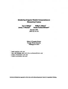
Figure 1: Mapping a mesh graph to a DAG via a second-order Hilbert curve. Grid points in the discretized Hilbert curve are numbered in black. Each vertex v is mapped to its closest grid point H (v), then the input graph is reordered according to this mapping: if H (v) < H (w ) for v, w ∈ V , then v appears before w in the reordered output. Ties between vertices mapped to the same grid point are broken randomly.

REORDERING VERTICES

In this section, we improve the theoretical upper bound on the miss rate of an M-vertex cache during a traversal of a Hilbertreordered random cube graph, tightening it from O(M −1/4 ) in [29] to O(M −1/3 ). We include evidence that the new O(M −1/3 ) bound is tight in practice, then build a generalized empirical model that accurately estimates the miss rate of a traversal of arbitrary-volume tetrahedralized mesh graphs [28].

2.1

0

Reordering with a Hilbert curve

To reorder a 3D mesh graph with a k-th order Hilbert curve, we first normalize the graph such that the 3D unit cube becomes its bounding box. We then divide up the unit cube into 2k × 2k × 2k equal-sized blocks, numbered according to the k-th order Hilbert curve. Figure 1 depicts the 2D analog of this process, for k = 2. Finally, we assign each vertex to the block that encloses its position in 3D space, then sort the vertices in linear time using a counting sort. We aim for each of the 23k blocks to contain O(1) vertices; frequently, simply setting k such that 23k = O(|V |) will suffice. For input graphs with highly non-uniform vertex density, simply choosing a value of k appropriate for the highest-density region would suffice. Setting k to an unnecessarily high value is not a concern, since it has minimal negative impact:

Figure 2: Theoretical upper-bounds and empirical measurements of cache miss rates during a traversal of the input graph across four different sizes of random cube graph, from 20MB (thinnest line) to 1.3GB (thickest line), as detailed in Section 4. Vertical lines show our test system’s memory hierarchy — the three lines correspond to one core’s share of the total L1, L2 and L3 cache capacity of our 48-core system, respectively. We show a per-core share even of the shared L3 cache (LLC), since all cores in a parallel execution load data into cache and must therefore share the space in the LLC. Hilbertreordering significantly reduces the number of cache misses across all input and cache sizes, and our improved upper bound on the cache miss rate is significantly tighter than the prior bound in [29].

• Computations on such a reordered input graph are no less efficient than ones with a more appropriate value of k. • Increasing k does not meaningfully increase the reordering process’ runtime, since assigning vertices to locations on the Hilbert curve is an embarrassingly parallel problem, and therefore the sorting operation dominates the reordering runtime. • Even on the largest (5.4GB, 27M vertex) input graphs, the reordering process takes no more than 10s — a trivial amount of time compared to the thousands of seconds required for the data-graph computation to reach convergence.

2.2

Improved expected miss rate bound

Recall that the l p norm of a vector t® = (t 1 , t 2 , . . . , tm ) is: ⎧ m |t | ⎪ for p = 0 i ⎨i=1 ⃦⃦ )︀1/p (︀ p p p ⃦t®⃦p = |t 1 | + |t 2 | + . . . |tm | for 0 < p < ∞ ⎪ ⎩ |t | maxm for p=∞ i i=1

We approximate the cache behavior of the computation with a traversal of the graph that visits each vertex in order. With an M-vertex cache, at each vertex v the cache contains all vertices in the range [v − M/2, v + M/2). Any neighbor of v outside that range would incur a cache miss. We can see in Figure 2 that reordering the vertices results in significantly lower cache miss rates across all cache sizes M. We also see that the miss rate as a function of the cache size is better captured by our tighter O(M −1/3 ) bound than the prior O(M −1/4 ) bound in [29].

Definition 1. The position x®v of each vertex v in an n-vertex random cube graph is chosen uniformly randomly in the unit cube and the edge set E = {(u, v) ∈ V × V : ∥x®u − x®v ∥p < r } connects vertices within non-negative l p distance r .

417

Session 10


The expected degree of a vertex v in a random cube graph is at most the expected number of vertices that fall within a ball of radius r . Since the vertices in G are distributed uniformly randomly in the unit cube, the expected degree of a vertex is equal to the volume of the radius r ball in the l p norm times the number of potential neighbors |V |. Consider a vertex v in a sub-cube C of size 2−j × 2−j × 2−j for some j, within the unit cube and aligned with the recursive decomposition of the space-filling curve, as depicted in Figure 3. We calculate the probability that another vertex w in the random cube graph is connected to v, yet lies outside C.

Definition 2. Given a graph with n vertices and cache size ∈ N, (︁define the minimum j such that √︁ j M ∈ (︀ N as )︀)︁ M ≥ 2−3j n 1 + (9 ln n)/ 2−3j n . M

and M ≥ 100 ln n, then √︁ Lemma (︀2. Given)︀a graph with n vertices √ (9 ln n)/ 2−3j M n ≤ 1 and 2j M ≤ 3 16n/M. √︁ (︁ (︀ )︀)︁ Proof. As M < 2−3(j M −1)n 1 + (9 ln n)/ 2−3(j M −1)n (otherwise, j M would not be minimal) and 100 ln n ≤ M, we have −3j M n > 9 ln n by a quadratic inequality manipulation and thus 2√︁ (︀ )︀ (9 ln n)/ 2−3j M n ≤ 1. Factoring out 8, we have (︁ (︀ )︀)︁ √ √︁ M < 8 · 2−3j M n 1 + 1/8 (9 ln n)/ 2−3j M n < 16 · 2−3j M n, and √ thus 2j M ≤ 3 16n/M. □

r

p

Lemma 3. Given an M-vertex cache and a random cube graph G = (V , E) divided into 2−j M ×2−j M ×2−j M sub-cubes, the probability that any sub-cube holds more than M vertices is at most |V | −2 for all M ≥ 100 ln|V |.

1

Vcap s

q 1

Proof. Let Xv be an indicator variable which indicates that vertex v is in a particular sub-cube√︁C. Let n = |V | and X = v Xv . (︀ )︀ Set µ = E [X ] = 2−3j M n and σ = (9 ln n)/ 2−3j M n (σ ≤ 1 by Lemma 2), then apply the Chernoff bound [8]: (︀ )︀ Pr {X ≥ (1 + σ )µ} ≤ exp −σ 2 µ/3 ∀σ ∈ [0, 1].

13 2−j

r C

Figure 3: The sub-cube C at H(13) of Figure 1, with three vertices s, p, and q with a different distance to the border. The probability that another vertex is placed outside of C, but within a radius r , is equal to the volume of the corresponding spherical cap Vcap .

Combining with the definition of j M , we get that Pr {X ≥ M } ≤ n −3 . There are at most n sub-cubes, so by the union bound, the probabil−2 ity that any hold more than M vertices is at most n·n −3 = |V | . □ Theorem 4. For any cache of M ≥ 100 ln|V | vertices and random cube graph G = (V , E) with l p distance parameter r such that E [|E|/|V |] = d is constant, a traversal of G, reordered using a Hilbert curve, incurs O(M −1/3 ) expected misses per vertex.

with l p

Lemma 1. Let G = (V , E), a random cube graph distance parameter r , be decomposed into a grid of 2j × 2j × 2j sub-cubes. The expected number of total edges connecting vertices in different sub-cubes is at most 6r 4 |V | 2 2j .

Proof. Let n = |V |. Let Ci be the number of vertices held by the ith sub-cube. If Ci < M ∀i, then all neighbors within a subcube would hit in the cache, so the number of misses is at most the expected number of edges connecting vertices in different subcubes, which is itself at most 6r 4n2 2j M by Lemma 1. The {︀ probability }︀ that not all sub-cubes hold fewer than M vertices Pr Ci < M ∀i is at most n −2 by Lemma 3, and as the number of edges is at most n 2 , the expected number of total misses is at most

Proof. Consider two vertices v and w; let v be in sub-cube C. The probability that w is placed within a distance r of v, yet outside C, is equal to the fraction of the volume of the radius-r ball under the l p norm centered on v that lies outside of C. This volume is at most the sum of the volume of the spherical caps — the section of a ball on one side of a plane intersecting the ball — that lie outside of C. We first consider a single face of C: let the spherical cap be centered a distance of h from the particular face of C. Recall that, since a ball in the l ∞ norm is a cube, the corresponding spherical cap in l ∞ is a rectangular prism and across all l p has maximal volume: 4r 2 (r − h). Therefore, for any l p , Vcap (h) ≤ 4r 2 (r − h) for h ∈ [0, r ], and Vcap (h) = 0 elsewhere. As v is uniformly randomly located in −2j and marginalize h out, C, we multiply [︀ ]︀by the area of the face 2 getting E Vcap ≤ 2r 4 2−2j . Each sub-cube has 6 faces and there are 23j total sub-cubes, so by the union bound, the probability that a particular pair of vertices is connected but lie in different sub-cubes is then at most 6×23j ×2r 4 2−2j = 12r 4 2j . There are at most |V | 2 /2 pairs of vertices, so the expected number of edges crossing between different subcubes is 6r 4 |V | 2 2j . □

Pr {Ci < M ∀i} · 6r 4n 2 2j M + n −2 · n2 ≤ 6r 4n 2 2j M + 1. Dividing by n vertices and substituting 2, the ex(︀ using )︀ √ Lemma pected number of misses per vertex is O r 4n 3 n/M . The expected number of edges per vertex d in a random cube graph is equal to the volume of the radius-r ball under the l p norm, times the number of vertices n. To upper bound the number of expected misses, we find the maximum r across all norms such that the volume of the radius-r ball equals d.√This occurs when l p = l 1 and the volume is (4/3)r 3 , thus r ≤ 3 3d/(4n) for all l p . Since d = O(1), the expected number of misses per vertex is at most (︃ )︃ √︂ (︁ )︁ 3dn 3 3dn O = O M −1/3 . 4n 4nM □

418

Session 10

2.3


Generalizing to arbitrary volumes

To simulate graphs with complex volumes, we extend our analysis to random arbitrary-volume graphs. Definition 3. The position x®v of each vertex v in an n-vertex random cube graph is chosen uniformly randomly within a volume enclosed by a surface S and the edge set E = {(u, v) ∈ V × V : ∥x®u − x®v ∥p < r } connects vertices within non-negative l p distance r . Each such graph has a fill-factor ρ, the fraction of the unit cube that is occupied by the surface after scaling it so that the unit cube is the surface’s bounding cube. Theorem 5. Let G be a random arbitrary-volume graph filling a fraction ρ ∈ (0, 1] of the unit cube. (︁ Given a)︁cache of M ≥ 100 ln|V | vertices, for all l p and all r = O (ρ/|V |)1/3 , a traversal of G reordered (︁ )︁ using a Hilbert curve incurs O (1/ρ)M −1/3 misses per vertex.

Figure 4: Model estimates and empirical measurements of cache miss rates during a traversal of the bunny, dragon, and cube graphs described in Section 4. Estimates are calculated based on the input graph’s fill-factor, as described in Section 2.3. The empirical measurements closely follow the model’s estimates across all cache sizes.

Proof. Let the vertices of G lie within a volume enclosed by a surface S. We start with a random cube graph ordered using a Hilbert curve, and remove all vertices that lie outside the volume enclosed by S. Each removal of a vertex makes the distance between all remaining vertex pairs either stay the same or decrease by one. Thus the total expected number of misses of an M-vertex cache than with (︁(︀ is no more )︁ a (|V |/ρ)-vertex random cube graph, )︀√︀ O r 4 |V | 2 /ρ 2 3 |V |/ρM . Since G has |V | vertices, the expected (︁(︀ )︁ )︀√︀ number of misses per vertex is O r 4 |V |/ρ 2 3 |V |/ρM . To (︁maximize the )︁ expected number of misses, we maximize

simultaneously are in different chunks and in the same phase require atomic decrements — empirically, 1–2% of all edges for the maximal-sized graphs in Section 4. The remaining 98–99% of all edges do not require any scheduling computation whatsoever — this is how Laika avoids the bulk of the coordination overhead incurred by JP. Laika uses a sawtooth-like priority function (see Figure 5) to ensure that edges between vertices in a single chunk are directed to create forward dependencies. Vertices near the beginning of a chunk (e.g., v in chunk 3) may have successors at the end of the previous chunk (i.e., chunk 2) and so a backward dependency. Forward dependencies within the same chunk are implicitly satisfied by the serial processing of chunks. The proximity-preserving reordering causes many backward dependencies to fall in the opposite phase of an adjacent chunk, implicitly satisfying them.

r = O (ρ/|V |)1/3 , the value of r that would yield a (|V |/ρ)-vertex random cube graph with O(1) expected degree by (︁ Theorem 4.)︁Then, the expected number of misses per vertex is O (1/ρ)M −1/3 .

□

By plugging in the fill-factor ρ of a real-world graph into the above bound, we can estimate that graph’s expected cache miss rate. Figure 4 confirms that these predictions are quite accurate across a variety of real-world graph topologies.

3

Increasing Priority

THE LAIKA SCHEDULER

We now describe Laika, a new in-place DAG scheduling algorithm. While it still uses a dependency counter at each vertex, Laika intentionally limits the exposed parallelism in the computation, thereby eliminating up to 99% of the coordination overhead caused by atomic counter decrements.

3.1

Forward Dependencies

0 Chunks

1

Backward Dependencies

3

2

u

v

4 2b Vertices

Typical Neighborhoods

Laika algorithm

Figure 5: Visualization of the Laika scheduling algorithm. Hilbert proximity-preserving reordering makes the neighbors of the vertices labeled u and v predominantly lie in the shaded regions surrounding them (“typical neighborhoods”).

The algorithm breaks up the vertex array into contiguous chunks of size 2b . Following the rule of thumb defined in [10, p. 783] that a program with at least 10P parallelism should achieve nearly perfect linear speedup on P processors, we set b to the maximum integer such that |V |/2b > 10P. Chunks are equally divided in two phases. Phases are processed serially, and in each phase chunks are processed in parallel. A barrier between the two phases obviates the need to protect against a data race between neighboring vertices from different phases. Due to the proximity-preserving Hilbert reordering of the vertices, most of the neighbors of any vertex v are nearby in memory. Only edges between vertices that

Laika uses an explicit randomized work-stealing scheduler (Figure 6), to coordinate chunk processing among P workers. Workers claim work from a set of P heap-allocated concurrent queues, all of which are visible to all workers. Each worker executes the function Laika-Worker in parallel, coordinating their work through the work queues, Q[0:P-1], and a shared counter activeChunks initialized in the parent function Laika.

419

Session 10


In Figure 7, each worker independently counts the rounds of the data-graph computation and the two phases of each round. Each phase begins with all workers pushing the chunks that nominally “belong” to them into their respective queues, as implemented in the function Push-Chunks in Figure 8. For example, we assume without loss of generality that P evenly divides |V |, there are N = |V |/P chunks per worker and worker p pushes chunks [N · p, N · (p + 1) − 1] into Q[p] on line 9. Workers then independently steal work from randomly selected queues on line 11; a successful steal

retrieves the pair ⟨c, idx⟩, where c is a chunk and idx is the index of the next vertex in c to be processed, on line 14. The worker will work on chunk c, as implemented by the function ProcessChunk in Figure 8, until it either finishes the last vertex in the phase or it cannot proceed due to an unmet dependency. Let w be the next vertex to be processed in chunk c, and consider the case where it has a dependency counter greater than 0. The worker must prematurely stop processing c, and c is shelved. The worker indicates that c has been shelved by decrementing the dependency counter of w. Thus, when the last predecessor of w is processed, w’s dependency counter will be decremented to a value of −1, indicating that w’s chunk c had been shelved when w was the next vertex to be processed. Figure 8 shows that the function Process-Chunk(v, Q, b) sequentially processes each vertex in the chunk, starting with v, until it cannot proceed due to an unmet dependency, as detected by the two logical clauses on line 1. If v is ready for processing (i.e., all vertices in the set v.pred have been updated), then the user-supplied Update(v) function is called and the counter v.counter is reset to |v.pred|, on lines 2 and 3, respectively. If any post-decrement counter value w.counter equals −1, then w’s chunk had been previously shelved and is now re-enabled, and so must be pushed onto its work queue on line 8. Finally, Process-Chunk moves on to the next vertex on line 9 and tests if the new vertex marks the start of a new phase on line 10, in which case the function returns.

Laika(G, b, rounds) 1 2 3 4 5 6 7 8 9 10 11 12

let G = (V , E) parallel for v ∈ V N ′ (v) = {w ∈ N (v) : Same-Phase(w, v) ∧ Different-Chunk(w, v)} v.pred = {w ∈ N ′ (v) : ρ(w) < ρ(v)} v.counter = |v.pred| v.succ = {w ∈ N ′ (v) : ρ(w) > ρ(v)} P = Get-Num-Workers( ) Q = Allocate-Queues(P) activeChunks = 0 for p = 1 to P spawn Laika-Worker(G, Q, b, activeChunks, rounds, P)

Figure 6: The Laika data-graph computation scheduling algorithm. Different-Chunk(w , v) (︀ returns ⌊︀ ⌋︀True ⌊︀ iff⌋︀)︀ w and v are in different chunks i.e., w /2b , v/2b . SameTrue iff w and )︀v are⌋︀)︀in the same phase (︀Phase(w ⌊︀(︀ , v) returns )︀ ⌋︀ ⌊︀(︀ i.e., w mod 2b /2b−1 = = v mod 2b /2b−1 . The priority function and these two helper functions allow Laika to find, for each vertex v, the predecessor and successor vertex sets that require explicit dependency tracking.

Push-Chunks(Q, chunk, numChunks, start)

Process-Chunk(v, Q, b) 1 2 3 4 5

Laika-Worker(G, Q, b, activeChunks, rounds, P) 1 2 3 4 5 6 7 8 9 10 11 12 13 14 15 16

parallel for c = 0 to numChunks − 1 Push(Q, ⟨chunk + c, start⟩)

1 2

let G = (V , E) p = Get-Worker-ID( ) start[0] = 0; start[1] = 2b−1 end[0] = 2b−1 ; end[1] = 2b N = |V |/P for round = 1 to rounds for phase = 0 to 1 Atomic-Add(activeChunks, N ) Push-Chunks(Q[p], N · p, N , start[phase]) while activeChunks > 0 ⟨c, idx⟩ = Pop(Q[Rand( ) (mod P)]) if c , nil v = V [idx + c · 2b ] if Process-Chunk(v, Q[p], b) = = end[phase] Atomic-Dec(activeChunks) Barrier( )

6 7 8 9 10 11 12

while v.counter = = 0 or Dec-And-Fetch(v.counter) = = −1 Update(v) v.counter = |v.pred| for w ∈ v.succ if Dec-And-Fetch(w.counter) = = −1 ⌊︁ ⌋︁ c = w/2b

idx = w mod 2b Push(Q, ⟨c, idx⟩) v = v +1 if v ≡ 0 (mod 2b−1 ) return v return v

Figure 8: Helper functions for Laika. Push-Chunks merely pushes onto the work queues Q the range of chunks [chunk, chunk + numChunks − 1] “belonging” to the worker calling the function, each with the index within the chunk of its starting vertex, start. Process-Chunk attempts to make as much progress as possible on the chunk, starting with vertex v, until it either finishes the chunk, on line 10, or reaches a vertex whose counter value indicates unmet dependencies, on line 1. If another worker happens to satisfy v’s last dependency and perform the final decrement to v.counter, then Dec-And-Fetch will return −1, which indicates that all dependencies for v have been met.

Figure 7: The Laika-Worker function executed by each worker. Each worker independently maintains the round and phase number (lines 6 and 7) via a shared variable, activeChunks. Each chunk is initially pushed onto its corresponding work queue on line 9, and the shared counter activeChunks is incremented for each chunk on line 8.

420

Session 10

3.2


Theorem 9. Let G = (V , E) be a random cube graph with expected degree d. Let n = |V |. For any c > 0 and 0 ≤ b < lg n − 1, Laika with chunk size 2b executes an ordinary data-graph computation on G with span greater than e 2 (2d + 3(4 + c) ln n)2 2b with probability less than n−(2+c) .

Analysis of Laika

We make the reasonable assumption that the data-graph computation is ordinary — i.e. the Update(v) function executes serially in O(N (v)) time for all v ∈ V . Theorem 6. Laika is work-efficient for any ordinary data-graph computation on any graph G = (V , E).

Proof. Consider Laikb, an modification of Laika where the kth vertex from all chunks must be processed before the k + 1st vertex from any chunk. Laika is always at least as fast as Laikb, so it suffices to prove that Laikb satisfies the lemma. Laika randomly directs edges between vertices at equal positions within their chunks, so at each chunk position k, such dependent edges form the priority DAG G k of Lemma 8. Then, Laikb’s span will be less than the product of: • the maximum degree (as Update(v) is serial with |N (v)| work); • the maximum depth among the 2b random priority DAGs {G 1 , G 2 , . . . , G 2b }; and • the total number of priority DAGs, 2b . Let A∆ be the event that the maximum degree in G exceeds ∆ = 2d + 3(4 + c) ln n and let AG k be the event that the depth of the priority DAG G k exceeds e 2 ∆, for all k ∈ [1, 2b ]. The event A∆ ∩ {∀k AG k } would imply that the overall span of Laikb applied to G is at most e 2 (2d + 3(4 + c) ln n)2 2b , since ∆ > (4 + c) ln n when A∆ is true, as required by Lemma 8. We use De Morgan’s law to find the negation of this event, and following from Lemmas 7 and 8, we see that the probability of the event A∆ ∪ {∀k AG k } is at most n−(2+c) . □

Proof. Laika calls Update once per vertex per iteration, just as in the baseline serial execution. Furthermore, there are at most |E| calls to Dec-And-Fetch made on counters on line 5. Finally, shelving and reactivating a chunk costs O(1) work, and any vertex v can only cause at most one shelving, so the total cost of shelving chunks is O(|V |). Therefore, Laika performs O(|V | + |E|) work and is work-efficient. □ Lemma 7. Let G = (V , E) be a random cube graph with expected degree d. For any c > 0, the maximum degree maxv ∈V |N (v)| is greater than 2d+3(4+c) ln|V | with probability no more than |V | −(3+c) . Proof. Let r be the distance parameter of G — the radius of the sphere such that vertices within a distance r are connected by an edge. Consider a vertex v of G, and let X w be a indicator variable where X w = = 1 denotes the event that a vertex w is connected to vertex v. For any w , v, the probability of an edge between v and w is d/|V |. We use now the Chernoff bound [8] for deviations of more than 1 times the mean: Pr {D ≥ (1 + β) · E [D]} ≤ exp(−(β/3)E [D])

Corollary 10. Let n = |V |. With P = O(n/log2 n) workers, Laika produces linear expected speedup.

∀β > 1,

where D = w X w [10, p. 1203]. By definition, D = |N (v)|, and E [|N (v)|] = d. Let β = (d + 3(4 + c) ln|V |)/d. Then,

Proof. The expected work of one iteration of the datagraph computation is E [v ∈V |N (v)|] = d |V | = 2|E|. Let AS denote the event that the computation has span exceeding e 2 (2d + 3(4 + c) ln n)2 . By Theorem 9, this occurs with probability at most n −(2+c) , letting 2b equal 1. Thus, the expected parallelism (the ratio of work to span) is at least {︀ }︀ 2|E| + Pr {AS } · 1 ≥ Pr AS 2 e (2d + 3(4 + c) ln n)2 (︁ )︁ 2|E| ≥ 1 − n −(2+c) 2 + n −(2+c) · 1 e (2d + 3(4 + c) ln n)2 )︂ (︁ )︁(︂ 2|E| ≥ 1 − n −(2+c) − 1 e 2 (2d + 3(4 + c) ln n)2

Pr {|N (v)| ≥ 2d + 3(4 + c) ln|V |} ≤ |V | −(4+c) . We use the union bound across all |V | vertices to see that G has maximum degree greater than 2d + 3(4 + c) ln|V | with probability at most |V | · |V | −(4+c) = |V | −(3+c) . □ Lemma 8. Let G = (V , E) be a graph with maximum degree ∆, let nG = |V |, and let G ρ be a priority DAG induced on G by a random priority function ρ. For any c > 0, there exists a directed path of length e 2 · max{∆, (4 +c) ln n} in G ρ for any n ≥ nG with probability at most n−(3+c) .

= Ω(n/log2 n).

Proof. For any v 1 , v 2 , . . . , vk , p = ⟨v 1 , v 2 , . . . , vk ⟩ is a directed path in G ρ with probability at most 1/k! ≤ (e/k)k , by Stirling’s approximation [10, p. 57], There are at most nG ∆k paths in G — nG potential starting points, and at most ∆ potential neighbors of each vertex. By the union bound, G ρ can contain a directed path of length k ≥ e 2 · max{∆, (4 + c) ln n} with probability at most (︂ (︂ 2 )︂)︂ (︂ )︂ e∆ k e max{∆, (4 + c) ln n} nG ≤ nG · exp −k ln k e∆ ≤ nG · exp(−k) (︀ (︀ )︀)︀ ≤ nG · exp − e 2 max{∆, (4 + c) ln n}

Laika is a randomized work-stealing scheduler [5], so the expected runtime is at most the work O(|V | + |E|) divided by the number P of workers, plus the span e 2 (2d + 3(4 + c) ln n)2 . Constraining P to be less than the parallelism makes the first term dominate and thus Laika runs in O((|V | + |E|)/P) time. A similar analysis holds for smaller values of P and correspondingly larger values of 2b . □

≤ n−(3+c) . □

421

Session 10

4


EMPIRICAL EVALUATION

We compare Laika across four graph topologies against the serial baseline and four alternative parallel schedulers: BSP — A deterministic Jacobi-type scheduler that uses doublebuffering to avoid determinacy races [12]. BSP stands for bulk-synchronous parallel execution [31]. Locks — An in-place scheduler that simply updates all vertices in parallel with reader-writer locks for concurrency control, yielding a nondeterministic result [26]. Chroma — A chromatic scheduler that colors the graph and serially loops through the colors, updating all vertices of the given color in parallel without the need for mutual-exclusion locks or atomic operations [21]. JP — A parallel DAG scheduler [20] built on a recursive function that updates a vertex once all of its predecessors have been updated using atomic operations. These alternative schedulers satisfy at most one of the three properties outlined in our optimization strategy: Chroma and BSP exhibit synchronization-overhead minimization due to their efficient parallelization, while JP exhibits execution locality as it recursively executes neighboring vertices’ update functions. To evaluate Laika, we conduct four studies: Per-iteration runtime — A per-iteration runtime analysis shows that Laika maintains nearly-linear parallel speedup across input sizes and topologies, and is 6.97–12.60x faster per iteration than the alternative parallel schedulers. None of the alternative schedulers match Laika’s performance, even with Hilbert-reordered inputs. Scalability — We analyze the scalability of each scheduler by measuring its parallel speedup on 12, 24, 36, and 48 cores, as shown in Figure 13. On 48 cores, we measured a parallel speedup of 38.4x for Laika, whereas all other schedulers scale less well. BSP, in particular, only achieves 28.05x speedup on 48 cores, even with Hilbert-reordered inputs. We also corroborate our theoretical analysis in Section 2 by collecting hardware performance counters in each operating regime. Convergence rate — We present evidence supporting the conventional wisdom [3, 6, 30] that in-place executions generally require fewer iterations to converge than doublebuffered executions. Laika consistently converges faster in wall-clock time than alternative schedulers, including the double-buffered BSP scheduler. Idealized performance — We show that Laika captures 54% of the theoretical upper bound of available performance, as defined by an ideal scheduler that achieves perfect linear speedup over the serial baseline scheduler.

Figure 9: Comparison of per-iteration wall-clock runtimes for each scheduler, in geometric mean across all topologies of the largest (5.4GB) input graphs, and normalized to Laika’s runtime. For each alternative scheduler, the left bar (labeled “Hilbert inputs”) represents the scheduler’s performance when using Hilbert-reordered input data, while the right bar (labeled “Random inputs”) represents the performance when using the original input order of each graph. Laika’s per-iteration runtime is faster than any other scheduler, and remains 2.78–8.89 times faster than the other in-place schedulers even when they are provided Hilbert-reordered inputs.

chips with a total of 48 physical processor cores. While we were not able to disable hyperthreading on the system, we used the taskset command to prevent execution of experiment code on hyperthreads. We disabled transparent huge pages system-wide, as the associated kernel activity can introduce measurement errors. Amazon EC2 instances enable dynamic frequency scaling, and unfortunately do not allow this setting to be changed. Our code is available online [14]. We intentionally chose an Update function that is difficult to schedule efficiently, since it executes only 2.22 instructions per byte of data. Such an update function exposes scheduler overheads; in the absence of good cache locality the computation will quickly become memory-bound on even a few cores [32]. This update function also presents difficulty for in-place execution, as the doublebuffered execution requires only 1.1–1.5 times as many iterations compared to an in-place execution. For comparison, this iterations ratio can be as high as 8x for some multigrid method [6] computations. Our Update function performs a physical simulation named Mass-Spring-Dashpot [18], simulating a set of weights of unit mass (vertices) in 3D space, connected by springs (edges). Each vertex experiences air drag proportional to its velocity, as well as spring restoration forces under compression or tension. We used four different graph topologies, each in five different sizes between 20MB (100k vertices) and 5.4GB (27M vertices). Each size increases the number of vertices roughly by a factor of 4, while retaining an average of 11–15 edges per vertex. The graph topology named rand is a random cube graph. The graphs named dragon, bunny, and cube were generated using TetGen [28], a tetrahedralizing mesh refinement engine that converts a 2D surface mesh (e.g.,

Experimental setup We implemented Laika and the other schedulers with a similar level of performance engineering in Cilk and C++, compiled them with GCC 7.3.0 with with these switches: -fcilkplus -std=c++11 -O3 -Wall -m64 -march=native -mtune=native -pthread -ffast-math -fgcse-las. All tests were executed on an Amazon EC2 m5.24xlarge cloud instance, a dual-socket system consisting of two 2.5GHz Intel Xeon Platinum 8175 (Skylake) CPU

422

Session 10

Scheduler Laika


Size 20MB 80MB 330MB 1.3GB 5.4GB

T1,H /|E|

T48,H /|E|

T1,H /T48,H

11.39 11.31 15.87 12.61 11.93

0.83 0.48 0.40 0.31 0.31

13.80 23.72 39.25 40.47 38.41

Table 10: Geometric mean of Laika runtimes across all graph topologies for each Hilbert-reordered input size. T1 /|E | and T48 /|E | denotes the runtime, in nanoseconds, of one iteration with 1 and 48 workers, normalized by the number of edges in the input. T1 /T48 is the parallel speedup on 48 cores. The 20MB inputs fit within L2 cache, whereas the 80MB inputs fit within L3 cache. As soon as the input graph’s size exceeds L3 cache, Laika is able to capture over 80% of the perfect parallel speedup possible on 48 cores.

Scheduler

Graph

Laika

dragon bunny cube rand

T1,H /|E|

T48,H /|E|

T1,H /T48,H

12.26 11.58 12.32 11.58

0.29 0.34 0.29 0.32

42.00 34.06 41.76 36.45

T1,R T1,L

T48,R T48,L

T1,R T48,L

T1,H T1,L

T48,H T48,L

T1,H T48,L

Locks BSP Chroma JP Laika

8.51 5.79 6.32 4.29 6.38

12.60 8.64 9.67 6.97 9.60

326.78 222.57 242.59 164.64 245.28

2.60 0.74 1.68 1.36 1.00

2.78 1.04 4.45 8.89 1.00

100.25 28.38 64.39 52.36 38.41

Table 12: Relative speedup of Laika compared to alternative schedulers on the largest input set in geometric mean across all graph topologies. Tk ,R and Tk ,H refer to an execution using k workers of a Randomly or Hilbert-reordered input. Tk ,L refers to a k -worker execution of the Hilbert-reordered input graph using Laika.

serial baseline scheduler applied to Hilbert-reordered graphs. Finally, the cost of Laika’s in-place updates appear to be outweighed by BSP’s cost of accessing two copies of vertex state: Laika is actually 4% faster per iteration than BSP with Hilbert-reordered inputs, while enabling further wall-clock speedups due to the superior convergence properties of in-place updates. For instance, as discussed in Section 4.3, Laika fully converges (to a remaining fraction of graph’s initial energy of 1.18x10−8 ) on the largest rand input graph 28.6% faster than BSP.

Table 11: Laika runtimes across all graph topologies, using the largest, 5.4GB-sized input sets. The measurement column headings are equivalent to Table 10.

4.2

Scalability

Figure 13 illustrates Laika’s superior scalability compared to all other schedulers, even on Hilbert-reordered inputs. Laika continues to achieve linear speedup with as many as 48 cores, whereas BSP with Hilbert inputs is already straining to maintain linear speedup with only 24 cores. It is tempting to extrapolate that Laika would continue to scale well at least in a weak-scaling regime [15], while BSP has nearly saturated memory and cross-socket communication bandwidth and will have trouble scaling much further. Figure 13 hints that Chroma is already in this situation: even though Hilbert reordering improves its per-iteration wall-clock speed, it comes at a significant scaling penalty starting at 24 cores. We used the Linux perf stat utility to measure a variety of CPU performance countersand provide further insight into the differences in scalability across schedulers. We also measured the parallel speedup on 48 cores for unordered (random-order) and Hilbert-reordered inputs, and the relative speedup afforded by the reordering process; Table 14 shows our results. Without reordering, all schedulers show evidence of poor cache utilization as predicted in Section 2 — their parallel speedup is only 23.49–26.05x on 48 cores, while incurring 0.53–1.27 LLC misses per edge and roughly 0.5 dTLB misses per edge. The dTLB is a small cache of translations between virtual and physical memory. If the virtual address being loaded is not present in the dTLB, a “page walk” occurs. The page walk traverses a tree structure that resides in memory and is cached in the LLC, just as any other memory state — competing for cache space with the data of the application itself. Therefore, each dTLB miss imposes a high latency penalty and frequently causes additional LLC misses. Given unordered input, all schedulers except for JP tend to suffer over 1 LLC miss for each edge they read; JP’s recursive structure tends to reuse some cached vertex data regardless of input order, making it suffer only about half as many misses as the other schedulers.

a surface tessellated by triangles) into a corresponding 3D volume mesh tessellated by non-overlapping tetrahedra. All measurements ignore the time taken to read the graph input files from disk, and any time taken for Hilbert curve reordering of the input. For the largest input graphs, Hilbert reordering took less than 9 seconds, whereas merely reading the graph from disk took 27 seconds; both times are a negligible fraction of the hours of wall-clock time of computation required to reach convergence.

4.1

Scheduler

Per-iteration runtime behavior

We measured the per-iteration execution runtimes of each scheduler across different graph topologies and sizes to determine the speedup of Laika versus other in-place, deterministic schedulers (Chroma and JP), as well as the performance penalty of in-place updates and determinism relative to BSP and Locks, respectively. Using input graphs reordered with the Hilbert curve, Table 10 demonstrates how as soon as the graph is large enough to not fit in the system’s cache, Laika shows good parallel speedup; Table 11 indicates that this speedup is insensitive to the specific bounding volume and topology (i.e., bunny versus dragon). Table 12 shows that Laika, using a Hilbert-reordered graph, is significantly faster (6.97–12.60x) than any alternative scheduler running on a randomly-ordered graph, and yields a 222.57x speedup over the serial baseline. Even with Laika’s Hilbert curve reordering, all other in-place schedulers remain slower than Laika, as we see in Figure 9 and Table 12. Per iteration, Laika is 4.45 times faster than Chroma, 8.89 times faster than JP, and 2.78 times faster than Locks. As Laika outperforms the nondeterministic Locks scheduler, Laika’s cost of determinism is negative. Laika is also 28.38 times faster than the

423

Session 10


Scheduler

Locks BSP Chroma JP Laika

LLC Misses Edge

dTLB Misses Edge

R /H

R /H

1.27 / 0.154 1.08 / 0.132 1.17 / 0.655 0.53 / 0.165 1.10 / 0.149

0.514 / 5.50e-3 0.504 / 2.79e-3 0.517 / 2.25e-2 0.226 / 2.68e-2 0.509 / 4.86e-3

T1,R T48,R

T1,H T48,H

T48,R T48,H

26.05 25.62 25.00 23.49 25.71

36.85 28.05 16.12 5.67 36.45

4.71 8.85 2.36 0.77 9.36

Table 14: Speedup and hardware performance counter measurements of data-graph computation schedulers executing the MassSpring-Dashpot model with 48 workers on the maximal-sized rand graph. The data under the subheadings R and H is taken with a Random and Hilbert ordering, respectively. The “LLC Misses / Edge” and “dTLB Misses / Edge” columns show the average number of load and store misses per edge use per iteration. Laika with Hilbert ordering incurs fewer LLC and dTLB misses than any other in-place scheduler. For example, Laika incurs 4.4 times fewer LLC misses and 4.6 times fewer dTLB misses than Chroma.

Similarly, the spatial locality produced by the reordering cannot alleviate Chroma’s poor temporal execution locality — it still incurs 0.655 LLC misses per edge as it reads each vertex in the graph approximately once for every color needed to color the graph, typically 3–5 colors for mesh graphs. While this is enough to improve performance by a factor of 2.36 relative to using unordered input, it is not sufficient to ensure good scalability, as the high LLC miss rate consumes large amounts of memory bandwidth. In contrast, Hilbert-reordered inputs allows Locks, BSP, and Laika to achieve much better performance on 48 cores than with unordered input graphs. Because of their predominantly sequential vertex access pattern and Hilbert reordering, these schedulers now display good execution locality. In addition, BSP and Laika have minimal coordination (much less often than once per edge), while the once-per-edge coordination in Locks mostly consists of uncontended reader lock acquisitions. As Laika was explicitly designed with well-ordered input in mind, it exhibits the highest reorderingrelated performance gain (9.36 times). While Hilbert reordering somewhat relieves the memory bandwidth bottleneck suffered by BSP using unordered graphs, its scalability is ultimately limited by the fact that BSP’s double buffering execution reads twice as much vertex data as the in-order schedulers.

Figure 13: Scalability (achieved parallel speedup) of different schedulers as a function of the number of physical CPU cores of the execution, in geometric mean across all topologies of the largest (5.4GB) input graphs. The top plot represents the measured parallel speedup, while the bottom plot shows the achieved fraction of perfect linear speedup. Dashed lines (labeled ending in “Random”) correspond to schedulers using the original input order, whereas solid lines (labeled ending in “Hilbert”) correspond to schedulers using our proximity-preserving reordered graph. Laika shows better scalability than any other scheduler, even when the alternative schedulers are provided Hilbert-reordered inputs. Laika always captures 80%+ of the ideal parallel speedup, achieving 38.4x speedup on 48 cores. Meanwhile, BSP’s doubled memory usage, Chroma’s high cache miss rate, and JP’s expensive atomic instructions cause these three schedulers to only capture less than 60% of the ideal parallel speedup with 48 cores, even on Hilbert-reordered inputs.

Hilbert-reordered inputs significantly reduce all schedulers’ LLC and dTLB miss rates, as a consequence of the cache advantages examined theoretically in Section 2 and empirically measured as shown in Table 14. For example, Laika with Hilbert ordering incurs 7.38 times fewer cache misses and 104.73 times fewer dTLB misses, making it 9.36 times faster overall. Reordering also appears to render prefetchers more effective, likely due to a more regular memory access pattern. However, the lower miss rates do not benefit all schedulers equally, and may in fact make performance worse! The reordering cannot alleviate JP’s execution of expensive atomic decrements: the same recursive structure that improved its reuse of cached data now exacerbates memory contention between those atomic instructions, causing JP on 48 cores with Hilbert inputs to only achieve 77% of the performance of using unordered inputs.

4.3

Convergence rate

As our chosen physical simulation dissipates energy with each iteration via air drag on the moving point masses, it converges as the remaining kinetic energy in the system decreases to a small fraction of the total energy present at the beginning of the computation. We recorded the number of iterations and the required wall-clock runtime (up to 14 hours) for all schedulers to reach a given fraction of the initial energy in the system. We show part of these results on the largest (5.4GB, 27M vertices) rand graph in Figure 15: Laika (solid blue line) reaches any energy fraction significantly faster than any alternative scheduler (dashed lines), and remains faster to most energy levels versus the alternative schedulers running on Hilbert-reordered inputs (remaining solid lines). The colored markers denoting increments of 10,000 iterations in Figure 15 show

424

Session 10


Figure 15: Remaining fraction of initial kinetic energy, as a function of wall-clock time, for different schedulers on the 5.4GB (27M vertices) rand input graph. Dashed lines (labeled ending in “Random”) correspond to schedulers using the original input order of the graph. Solid lines (labeled ending in “Hilbert”) correspond to schedulers using our proximity-preserving reordered graph. For scale convenience, we stopped execution after six hours (21,600s) of wall-clock time. Colored markers denote multiples of 10,000 iterations for each scheduler, starting with the 10,000th iteration. Even on Hilbert-reordered inputs, all existing in-place schedulers take 2.6–8.8 times longer than Laika to reach any energy level.

that in any fixed number of iterations, all in-place schedulers reach almost the same energy fraction, regardless of implementation or input reordering. Furthermore, we see that for our physical simulation, all in-place schedulers exhibit superior per-iteration convergence rates compared to double-buffering: starting around energy fraction 3 × 10−6 (approx. 4000s into the experiment), the colored markers of BSP with Hilbert-reordered data start appearing at higher energy fractions than the corresponding markers of in-place schedulers. Even though Laika’s iterations are only 4% faster than BSP’s iterations with Hilbert inputs, this difference in per-iteration convergence rates widens the performance gap between them with every iteration. After 14 hours of wall-clock execution time, the energy fraction that BSP with Hilbert data reaches is one that Laika achieved in only 10.86 hours — a performance gap of 28.6%. This effect is not unexpected, since many computations experience faster periteration convergence with in-place execution compared to doublebuffering [3]. In fact, this difference in convergence rates in favor of in-place scheduling can be significantly higher than our physical simulation experiences — as high as 8x in some multigrid method computations [6].

4.4

overhead; its perfectly-linear parallelization yields our idealized scheduler. Thus, if T1,SB denotes the serial baseline’s runtime, the upper-bound on parallel performance with P processors is T1,SB /P, hence T48,Ideal = T1,SB /48. In practice, this performance level is unattainable since a serial execution makes use of the entire LLC, whereas a parallel execution requires cores to share the LLC. In geometric mean across all topologies of the largest, 5.4GB Hilbert-reordered input graphs, we calculate the ratio between the runtimes of Laika and the idealized scheduler: T48,Laika /T48,Ideal = 0.540. Therefore, Laika captures 54% of the theoretical upper-bound performance, while providing both determinism and in-place execution. BSP with Hilbert-reordered inputs captures 51.7% of the upper-bound, while sacrificing in-place execution and its potential convergence rate advantages discussed in Section 4.3. The other in-place schedulers, even with Hilbert-reordered inputs, fall short: Locks achieves only 19.4% of the upper-bound while sacrificing determinism, while Chroma and JP provide deterministic execution but only manage 12.1% and 6.07%, respectively.

5

CONCLUSION

Practical high-performance data-graph computations are a challenging problem because they require both performance-engineering and domain-specific expertise. Attempting to improve usability, projects like Simit [24] and Prism [21] abstract away the scheduler and require the practitioner to only implement a serial update function for their computation. While we believe this is a good model, we have shown that the ability to adapt the scheduler to the particular input and computation can result in further performance gains for a variety of schedulers — up to 9.36x speedup in the case of simply Hilbert-reordering a mesh graph input.

Idealized performance

To estimate the remaining potential for improvement upon Laika’s performance, we construct a theoretical model of an idealized scheduler that achieves perfect linear speedup, suffers no coordination overhead, and does no work other than executing update functions. Our idealized scheduler is a physical manifestation of the work law from work-span analysis [10, p. 780]: the serial baseline scheduler already performs no coordination and has no other scheduling

425

Session 10


Modular schedulers designed according to our three-step design strategy maximize performance by allowing practitioners to incorporate domain-specific expertise into the scheduler. For example, Laika relies on Hilbert curves for proximity-preserving reordering as we were able to prove their cache-efficiency on mesh graph inputs; however, with different inputs, one may wish to instead use a graph partitioning scheme like METIS [23], PT-Scotch [9], or Zoltan [7]. Similarly, if future research uncovers a more efficient technique for synchronization-overhead minimization, that part of the scheduler can be upgraded with minimal impact on the other scheduler components. Such modularity also allows schedulers to adapt to different hardware architectures. While this paper focuses on shared-memory data-graph computations, the same ideas can in principle be applied to, e.g., high-performance distributed computing systems: Synchronization-overhead minimization and spatial and temporal locality become even more important when the worst-case latency costs increase by orders of magnitude, from RAM access to network access. We look forward to further exploring the potential performance gains stemming from this flexibility in our future work.

[12] Mingdong Feng and Charles E. Leiserson. 1997. Efficient Detection of Determinacy Races in Cilk Programs. In Proceedings of the Ninth Annual ACM Symposium on Parallel Algorithms and Architectures (SPAA ’97). ACM, New York, NY, USA, 1–11. https://doi.org/10.1145/258492.258493 [13] Björn Gmeiner, Harald Köstler, Markus Stürmer, and Ulrich Rüde. 2014. Parallel multigrid on hierarchical hybrid grids: a performance study on current high performance computing clusters. Concurrency and Computation: Practice and Experience 26, 1 (2014), 217–240. https://doi.org/10.1002/cpe.2968 [14] Predrag Gruevski, William Hasenplaugh, and James J. Thomas. 2018. Laika: Efficient In-Place Scheduling for 3D Mesh Graph Computations. https://github. com/data-graph-computations/laika. [15] John L. Gustafson. 1988. Reevaluating Amdahl’s Law. Commun. ACM 31, 5 (May 1988), 532–533. https://doi.org/10.1145/42411.42415 [16] Gundolf Haase, Manfred Liebmann, and Gernot Plank. 2007. A Hilbert-order Multiplication Scheme for Unstructured Sparse Matrices. Int. J. Parallel Emerg. Distrib. Syst. 22, 4 (Jan. 2007), 213–220. https://doi.org/10.1080/17445760601122084 [17] Daniel F. Harlacher, Harald Klimach, Sabine Roller, Christian Siebert, and Felix Wolf. 2012. Dynamic Load Balancing for Unstructured Meshes on Space-Filling Curves. In Proceedings of the 2012 IEEE 26th International Parallel and Distributed Processing Symposium Workshops & PhD Forum (IPDPSW ’12). IEEE Computer Society, Washington, DC, USA, 1661–1669. https://doi.org/10.1109/IPDPSW. 2012.207 [18] William Hasenplaugh. 2016. Parallel Algorithms for Scheduling Data-Graph Computations. Ph.D. Dissertation. MIT. [19] David Hilbert. 1891. Über die stetige abbildung einer linie auf ein flächenstück. Math. Ann. (1891). [20] Mark T. Jones and Paul E. Plassmann. 1993. A Parallel Graph Coloring Heuristic. SIAM J. Sci. Comput. 14, 3 (May 1993), 654–669. https://doi.org/10.1137/0914041 [21] Tim Kaler, William Hasenplaugh, Tao B. Schardl, and Charles E. Leiserson. 2014. Executing Dynamic Data-graph Computations Deterministically Using Chromatic Scheduling. In Proceedings of the 26th ACM Symposium on Parallelism in Algorithms and Architectures (SPAA ’14). ACM, New York, NY, USA, 154–165. https://doi.org/10.1145/2612669.2612673 [22] Kab Seok Kang. 2015. Scalable Implementation of the Parallel Multigrid Method on Massively Parallel Computers. Comput. Math. Appl. 70, 11 (Dec. 2015), 2701– 2708. https://doi.org/10.1016/j.camwa.2015.07.023 [23] George Karypis and Vipin Kumar. 1998. A Fast and High Quality Multilevel Scheme for Partitioning Irregular Graphs. SIAM Journal on Scientific Computing 20, 1 (1998), 359–392. https://doi.org/10.1137/S1064827595287997 arXiv:http://dx.doi.org/10.1137/S1064827595287997 [24] Fredrik Kjølstad, Shoaib Kamil, Jonathan Ragan-Kelley, David I. W. Levin, Shinjiro Sueda, Desai Chen, Etienne Vouga, Danny M. Kaufman, Gurtej Kanwar, Wojciech Matusik, and Saman Amarasinghe. 2016. Simit: A Language for Physical Simulation. ACM Trans. Graph. 35, 2, Article 20 (March 2016), 21 pages. https://doi.org/10.1145/2866569 [25] Yucheng Low, Danny Bickson, Joseph Gonzalez, Carlos Guestrin, Aapo Kyrola, and Joseph M. Hellerstein. 2012. Distributed GraphLab: A Framework for Machine Learning and Data Mining in the Cloud. Proc. VLDB Endow. 5, 8 (April 2012), 716–727. https://doi.org/10.14778/2212351.2212354 [26] Yucheng Low, Joseph Gonzalez, Aapo Kyrola, Danny Bickson, Carlos Guestrin, and Joseph M. Hellerstein. 2010. GraphLab: A New Parallel Framework for Machine Learning. In Conference on Uncertainty in Artificial Intelligence (UAI). Catalina Island, California. [27] Bongki Moon, H. V. Jagadish, Christos Faloutsos, and Joel H. Saltz. 2001. Analysis of the clustering properties of the Hilbert space-filling curve. IEEE Transactions on Knowledge and Data Engineering 13 (2001), 2001. [28] Hang Si. 2015. TetGen, a Delaunay-Based Quality Tetrahedral Mesh Generator. ACM Trans. Math. Softw. 41, 2 (January 2015). [29] Srikanta Tirthapura, Sudip Seal, and Srinivas Aluru. 2006. A Formal Analysis of Space Filling Curves for Parallel Domain Decomposition. In Proceedings of the 2006 International Conference on Parallel Processing (ICPP ’06). IEEE Computer Society, Washington, DC, USA, 505–512. https://doi.org/10.1109/ICPP.2006.7 [30] John N. Tsitsiklis. 1989. A comparison of Jacobi and Gauss-Seidel parallel iterations. IEEE Trans. Aut. Control 2 (1989), 325–332. [31] Leslie G. Valiant. 1990. A Bridging Model for Parallel Computation. Commun. ACM 33, 8 (Aug. 1990), 103–111. https://doi.org/10.1145/79173.79181 [32] Samuel Webb Williams, Andrew Waterman, and David A. Patterson. 2008. Roofline: An Insightful Visual Performance Model for Floating-Point Programs and Multicore Architectures. Technical Report UCB/EECS-2008-134. University of California at Berkeley. [33] Albert Jan Nicholas Yzelman and Dirk Roose. 2014. High-Level Strategies for Parallel Shared-Memory Sparse Matrix-Vector Multiplication. IEEE Transactions on Parallel and Distributed Systems 25 (Jan 2014), 116–125. https://doi.org/10. 1109/TPDS.2013.31 [34] Jinshan Zeng, Zhimin Peng, and Shaobo Lin. 2015. A Gauss-Seidel Iterative Thresholding Algorithm for lq Regularized Least Squares Regression. CoRR abs/1507.03173 (2015). http://arxiv.org/abs/1507.03173

ACKNOWLEDGMENTS We would like to thank Charles E. Leiserson, Tao B. Schardl, and Tim Kaler from the Supertech group at MIT. They continue to be very generous with insights, humor, and technical assistance. We would like to thank Fredrik Kjølstad who inspired us to schedule data-graph computations on 3D mesh graphs and provided much needed context on real applications. Thanks to Leonid Taycher at Kensho Technologies for his patience, support, and understanding while this work was in progress. This work is sponsored in part by the Direction Générale de l’Armement, Kensho Technologies, and MIT’s SuperUROP program; we thank them for their support.

REFERENCES [1] L. Adams and J. Ortega. 1982. A multi-color SOR method for parallel computation. In International Conference on Parallel Processing. 53–56. [2] Mark Adams, Marian Brezina, Jonathan Hu, and Ray Tuminaro. 2003. Parallel Multigrid Smoothing: Polynomial versus Gauss-Seidel. J. Comp. Phys 188 (2003), 593–610. [3] Mark F. Adams. 2001. A Distributed Memory Unstructured Gauss-Seidel Algorithm for Multigrid Smoothers. In Proceedings of the 2001 ACM/IEEE Conference on Supercomputing (SC ’01). ACM, New York, NY, USA, 4–4. https: //doi.org/10.1145/582034.582038 [4] Dimitri P. Bertsekas and John N. Tsitsiklis. 1989. Parallel and Distributed Computation: Numerical Methods. Prentice-Hall, Upper Saddle River, NJ, USA. [5] Robert D. Blumofe and Charles E. Leiserson. 1999. Scheduling Multithreaded Computations by Work Stealing. J. ACM 46, 5 (1999), 720–748. https://doi.org/ 10.1145/324133.324234 [6] William L. Briggs, Van Emden Henson, and Steve F. McCormick. 2000. A Multigrid Tutorial. SIAM: Society for Industrial and Applied Mathematics. [7] Ümit V. Çatalyürek, Erik G. Boman, Karen D. Devine, Doruk Bozdag, Robert Heaphy, and Lee Ann Riesen. 2007. Hypergraph-based Dynamic Load Balancing for Adaptive Scientific Computations. In Proc. of 21st International Parallel and Distributed Processing Symposium (IPDPS’07). IEEE. [8] Herman Chernoff. 1952. A Measure of Asymptotic Efficiency for Tests of a Hypothesis Based on the sum of Observations. The Annals of Mathematical Statistics 23, 4 (1952), 493–507. [9] Cédric Chevalier and François Pellegrini. 2008. PT-Scotch: A tool for efficient parallel graph ordering. Parallel Comput. 34, 6 (2008), 318 – 331. Parallel Matrix Algorithms and Applications. [10] Thomas H. Cormen, Charles E. Leiserson, Ronald L. Rivest, and Clifford Stein. 2009. Introduction to Algorithms, Third Edition (3rd ed.). The MIT Press. [11] D. J. Evans. 1984. Parallel S.O.R. Iterative Methods. Parallel Comput. 1, 1 (Aug. 1984), 3–18. https://doi.org/10.1016/S0167-8191(84)90380-6

426