sensors Article
Landmark-Based Homing Navigation Using Omnidirectional Depth Information Changmin Lee, Seung-Eun Yu and DaeEun Kim * School of Electrical and Electronic Engineering, Yonsei University, 50 Yonsei-ro, Seodaemun-gu, Seoul 03722, Korea;
[email protected] (C.L.);
[email protected] (S.-E.Y.) * Correspondence:
[email protected]; Tel.: +82-2-2123-5879 Received: 22 June 2017; Accepted: 18 August 2017; Published: 22 August 2017
Abstract: A number of landmark-based navigation algorithms have been studied using feature extraction over the visual information. In this paper, we apply the distance information of the surrounding environment in a landmark navigation model. We mount a depth sensor on a mobile robot, in order to obtain omnidirectional distance information. The surrounding environment is represented as a circular form of landmark vectors, which forms a snapshot. The depth snapshots at the current position and the target position are compared to determine the homing direction, inspired by the snapshot model. Here, we suggest a holistic view of panoramic depth information for homing navigation where each sample point is taken as a landmark. The results are shown in a vector map of homing vectors. The performance of the suggested method is evaluated based on the angular errors and the homing success rate. Omnidirectional depth information about the surrounding environment can be a promising source of landmark homing navigation. We demonstrate the results that a holistic approach with omnidirectional depth information shows effective homing navigation. Keywords: landmark navigation; homing navigation; distance sensor; distance-estimated landmark vector; landmark vector; arrangement order matching
1. Introduction A number of methods have been developed for the challenging issue of autonomous navigation of mobile robots [1–5]. The methods vary widely, from landmark-based navigation [6,7], which is inspired by insect homing behavior, to complex algorithms that require intensive computation and continuous tracking of the information about the environment [1,8–10]. In homing navigation methods, the agent can assess an environmental feature obtained at the current position and can compare it to that at a target position. By comparing the feature information at two locations, the agent can determine which direction to move in to reach the target position. This concept has been proposed as the ‘snapshot model’ [11–13]. A snapshot taken at the current location is compared with a snapshot at the home location to obtain the direction from the current position to the home location. Various methods have been suggested for homing navigation, and among them, we focus on homing algorithms that are based on the snapshot model. One snapshot method, the warping method [14,15], distorts the current snapshot image in order to best match the target snapshot image. The agent predicts a new image for every possible direction that it could move from the current location by warping the snapshot image. Each warped image is compared to the target image by searching for the one with the smallest discrepancy. The warped image with the smallest difference indicates the direction in which to move in order to reach the target location. The performance of the predictive warping method is largely affected by the characteristics of the environment and the existence of a reference compass; however, the method is simple and does not require any pre-processing of feature extraction in the snapshot image.
Sensors 2017, 17, 1928; doi:10.3390/s17081928
www.mdpi.com/journal/sensors
Sensors 2017, 17, 1928
2 of 24
The Descent in Image Distance (DID) method extends the concept from the warping method. The DID method was introduced by Zeil et al. and was investigated from various perspectives [16,17]. While the one-dimensional warping method only searches for the minimum difference from the home image among the candidate images, the DID method monitors variations of the image difference between a pair of locations. The difference between snapshots decreases as the location becomes closer to the home point. By applying a gradient descent method, the navigation algorithm successfully finds the direction to the goal location [15,18]. One of the simplest homing navigation methods is the Average Landmark Vector (ALV) model [6]. At each location, the mobile robot takes a snapshot image, and each landmark in the view composes a landmark vector. Each landmark vector has a unit length with an angle as the corresponding angular position of the landmark. The ALV is computed by averaging all of the landmark vectors. The ALV computed at an arbitrary position is compared to that at the home location. By comparing only two averaged landmark vectors, the agent can determine the appropriate direction to the home location. Therefore, this navigation method has a small computing time and requires a small amount of memory. This method shows good homing navigation performance using a simple representation of the surrounding environment [19]. The Distance-Estimated Landmark Vector (DELV) model is another landmark-based homing navigation algorithm [20]. While the ALV model produces and compares two ALVs at different positions, the DELV method compares two sets of landmark vectors in order to determine the homing direction. These two navigation algorithms share similar concepts of landmark vectors, pointing to landmarks at a given position. However, while the landmark vectors in the ALV model have a unit length, DELV includes the length of the vector as the estimated distance to each landmark. Thus, the DELV method possesses more detailed information about the surrounding environment around the agent through the use of distance-estimated landmark vectors, and as a result, the agent estimates the current location with respect to the home location. In addition, the matching process of the landmark vectors in the DELV model does not require the reference compass information, while the ALV model necessarily does. The DELV model was initially tested using vision sensors, so an additional distance estimation process is required for selected landmarks [21,22]. Based on the visual information, variations in the landmark position between snapshots obtained at a sequence of robot positions can lead to the computation of the landmark distance. However, by exploiting the depth sensor, the distance information to each landmark can be given along with the landmark selection. Extracting the landmark feature may be a painful procedure, since in some cases, the accurate identification of each landmark and the determination of what landmarks should be selected in a real environment are non-trivial problems. The homing performance with DELV or ALV becomes much worse in a real environment than in an artificial environment with clearcut landmarks. The localization issue is a challenging issue, even in modern Simultaneous Localization And Mapping (SLAM) technology. Information about the environment can also be obtained from several types of sensors. The global localization map can be obtained with a global positioning system (GPS) and a laser-ranging sensor. The laser range sensor can also be tested for human robot interaction [5] or industrial applications [23]. In addition to the distance information about the environment, the Monte Carlo approach with an elevation map of objects or three-dimensional features commonly observed from the air and ground can be used to provide better localization information [24,25]. The landmark-based methods described above collect particular features called landmarks, and the snapshot model simplifies the navigation issue into the homing navigation. A mobile robot needs no localization map with the landmark-based method and thus the method efficiently determines the homing directions without identifying the current location. However, a high level of knowledge such as the environmental map cannot be obtained. In contrast, the SLAM method can utilize the localization map to guide a specific goal position with more computing time and memory.
Sensors 2017, 17, 1928
3 of 24
Visual information has been most widely applied to navigation algorithms, since it can provide a lot of information about the position, brightness, color, and shape of objects. Many navigation algorithms are developed with feature extraction using vision [26–28], often with a complex filtering process [29]. Even simple landmark-based navigation methods, including the ALV model, have been applied to a mobile robot with vision sensors, and a feature extraction process to identify landmarks is also required [26]. In contrast, the DID method is a holistic approach for comparing a pair of snapshot images pixel by pixel to calculate the image distance [15–17]. It has no feature extraction process; however, computing the gradient of the image distance is needed to determine the homing direction. The main contribution of this paper is in suggesting a holistic approach with the omnidirectional depth information including the background for homing navigation in a real environment, which is called H-DELV. It is a landmark-based navigation with distance information, but an effort of extracting landmark features can be omitted with the suggested approach. We assume that the environment roughly has an isotropic landmark distribution where the frequency of landmarks are independent of the viewing direction and the majority of landmarks are commonly observed irrespective of the view. We explore the efficient and robust landmark-based navigation of a mobile robot without prior knowledge of landmarks such as the colors or shapes of landmarks. We will show that one-dimensional panoramic distance information is sufficient to localize the agent in the environment to guide the homing performance. We suggest a holistic approach of reading landmarks using omnidirectional depth information for homing navigation in a real environment. In our experiments, we test the homing navigation based on landmark segmentation over the depth information, as well as that based on a holistic view of the depth information. We analyze the effect of landmark vector strategies using data from various experiments, changing the weight of landmark vectors, using the reference compass or not, varying the number of landmark vectors, and adding the feature extraction or clustering process. Our paper seeks answers to the following questions: What are important factors that influence the homing performance in the snapshot model as a bio-inspired model? What kind of landmark vector strategies will be useful if the distance sensor readings are available? What strategies will be helpful in an environment assuming an isotropic landmark distribution? Which strategy, a holistic view of landmarks or a landmark distribution involved with the feature extraction, will be more effective in real environments? Is the robotic homing model similar to the model for insect navigation? 2. Methods Initially, we explain the robotic configuration for homing navigation. From the depth sensor, omnidirectional depth information as the depth snapshot is obtained by following the snapshot model. How landmarks are extracted in the snapshot determines which landmark vector strategies can be used. We will introduce two new approaches based on the landmark distance vectors, C-DELV and H-DELV and compare those with the conventional DELV method. In this section, we will explain the three methods one by one. 2.1. Mobile Robot with a Depth Sensor For our navigation experiments, a mobile robot was used with a distance sensor as shown in Figure 1a. The mobile robot (Roomba, Create 4400, iRobot, Bedford, MA, USA) is a two-wheeled robot that can control the motor speed. A laptop computer processing the sensor readings from a laser sensor or vision sensor was connected to the robot via serial port for motor control. Depth information was obtained with a laser sensor device (URG-04LX-UG01, HOKUYO, Osaka, Japan)mounted on top of the Roomba with an acrylic support. The laser sensor can read distance information from the environment, which is then transmitted to a laptop computer on the robot. Figure 1b shows an example of distance sensor readings, where red x marks with an interval of angular resolution indicate detection points. In addition, one object makes some occlusion area on the wall which is marked in pink. The depth sensor has a distance accuracy of 5 mm (within a range of 60–1000 mm) or 30 mm
Sensors 2017, 17, 1928
4 of 24
(within a range of 1000–4095 mm) and an angular resolution of about 0.36◦ . We collect omnidirectional distance information for one snapshot at a given location, that is, a set of distances for the whole range of angles.
(a)
(b)
Figure 1. Mobile robot and sensor reading example (a) a mobile robot Roomba robot mounted with a laser sensor as the depth sensor; (b) an example of sensor readings with the laser sensor (red x marks show the distance readings for given angles).
The computer processes a landmark-based algorithm and transfers the appropriate motor actions to the robot. For a panoramic image (depth map) of the surrounding environment, the mobile robot takes two snapshots at a given location using the laser sensor, since the laser sensor has a limited viewing angle, 240◦ for a snapshot. The 360◦ omni-directional depth information was obtained by overlapping the two snapshots. The mobile robot Roomba runs with its own battery pack and it can sustain for a period of 1.5 h (on a hard floor with no payloads or attachments) when the robot constantly moves. The laptop computer has a separate battery pack that also supplies power (about 2.5 Watts) for the depth sensor with USB connection. The laptop computer uses MATLAB software (MATLAB, 2014b, MathWorks, Natick, MA, USA) to run the control algorithm and consumes 7–11 watts. With the batteries, the whole system can operate for about an hour. To check the performance in terms of the homing direction, we used a regular grid of points on the floor as well as additional random positions to see the performance, where small markers were placed for easy detection. The robot was manually positioned at each of those points to sense the surrounding environment and the robot estimated the homing directions, using the suggested snapshot model algorithm. 2.2. Depth Information Processing The experimental environment is a 3 m × 3 m area containing objects such as a desk, drawer, and trash bin. The panoramic depth information obtained with a mobile robot is shown in Figure 2. By using the depth information for a certain height of the view, we obtain a one-dimensional depth snapshot. Only this one-dimensional snapshot will be used as the environmental information for our navigation experiments. Figure 3 shows examples of the depth snapshot, which has 720-pixel width with a resolution of 0.5◦ . Since we only sample distance information at a certain height, it may not represent all of the information about every landmark in the environment. However, we assume that it can give sufficient information about the landmarks in terms of the mobile robot’s view, especially for our navigation experiments.
Sensors 2017, 17, 1928
5 of 24
(a)
(b) Figure 2. Test environments (a) environment env1 (left: environment, right: distance map at the home location with a laser sensor, *: home location); blue lines: top-view of objects, green dashed rectangle: interest zone for test points, called Region 2, black arrow: the reference direction (zero degree). The laser sensor collects the range data in a counterclockwise direction, and red x marks indicate detection points read by the laser sensor; (b) environments, env2 (left) and env3 (right) (O1 , ..., O5 : objects).
Depth difference, dv/dx Depth information v
650
500 400
O3
O4
O2
O1
O2
O3
O
4
580
300 200 100
510
0
90
180
270
O3
360 Region 1
440
200 100 0 -100 -200
Region 2 370 O
1
0
90
180
Angular position, x
270
360 300 300
370
440
510
580
650
Figure 3. Example of depth snapshot (left: depth snapshot for env1 and the derivative of the depth, right: close landmark objects (blue circles with labels) extracted from the depth snapshot). Black rectangles with label ‘Region 1’ and ‘Region 2’ (green dashed rectangle in Figure 2) include testing points.
Sensors 2017, 17, 1928
6 of 24
In our experiment, the DELV method [21] will be tested for landmark-based navigation. In order to use the DELV method, certain ‘landmarks’ should be selected. A set of landmarks can be obtained from segmenting the depth information. This pre-processing for a set of landmarks has been tested with vision [21]. Using visual information, objects can be found with image pixels based on similar color and the brightness, that is, by a feature extraction algorithm with clustering. Using the depth information, two main criteria were used for the landmark extraction. The first criterion is based on the difference of the depth values. The differences of the distance value between neighboring points in the panoramic snapshot are calculated. Since the boundaries of the landmarks would have large variations in their depth values, we set points with large difference as the preliminary landmark boundaries. Assuming continuity of the depth values in each landmark, candidate areas for the landmarks are selected. The second criterion is the threshold value of the depth information. Within the preliminary landmark area set by the first criterion, several regions with small depth values (small distances) are selected as landmarks. An example of depth snapshot and the corresponding landmark extraction results are shown in Figure 3. Left figures of Figure 3 show the depth values for the 360◦ surroundings of a mobile robot at the home location and its derivatives (for edge detection). The candidates were selected based on the points with large depth derivatives. Comparing the position of the selected landmarks and the depth information, we can observe large variations at the boundaries of the landmarks and comparatively small variations inside the landmark areas. The objects closer to the agent were selected prior to the background areas, using the thresholding value in the second criterion. If the location is closer to the wall than to the other objects, the agent could regard the wall area as one of the landmarks. 2.3. Navigation Algorithm: DELV For the snapshot navigation, we initially tested the Distance-Estimated Landmark Vector (DELV) model [21], which is an efficient landmark-based homing navigation algorithm. Each landmark vector in the DELV method has information about an angular position of the landmark, given as the angle of the vector, with the distance to the landmark as its length. The landmark vectors obtained at the home location create a reference map. The set of landmark vectors at an arbitrary location is projected on the reference map with an appropriate arrangement order and direction (see Figure 4). The landmark vector order and the heading direction are estimated by rotational projection of vectors. When the landmark vectors are appropriately matched with the corresponding ones in the reference map, that is, with the right order of landmark vectors, the end points of the projected landmark vectors would converge to the current location. In other words, we can find the appropriate landmark arrangement order by monitoring the deviation of the projected end points. The arrangement order with the minimum deviation of end points would indicate the appropriate matching. In the same way, we can project the landmark vectors by rotating the heading direction and estimate the current heading direction in the reference map, if there is no reference compass available. Ultimately, the above landmark arrangement process determines the homing direction. Here, we suggest two new methods, C-DELV and H-DELV that have different landmark vectors from the depth snapshot.
Sensors 2017, 17, 1928
7 of 24
LV 1 LV 2
LV 1
LV 3 LV 3 LV 2 LV 1
LV 3
(a)
LV 2 (b)
(c)
Figure 4. Projecting landmark vectors onto the reference map in different arrangement orders, and the correct order can be determined with the deviation of end points of projected landmarks ((a) for the best matching case, and (b,c) for other matching cases).
2.4. Navigation Algorithm: C-DELV Method The DELV method collects landmarks by assigning one representative landmark vector for each landmark area or segmented region. The centroid of the angular positions of points in the landmark area and the average of the depths of the points are the angle and the distance for a landmark vector. In this way, we obtain one landmark vector for each selected landmark area. For example, in Figure 3a, there would be four landmark vectors at a given position. Here, the size of landmark areas is not considered for the landmark representations. Now, we consider another type of landmark representation from a depth snapshot. The landmark representation defines every point in the landmark area as the individual landmark vector, but the background area is ignored. Only dominant landmarks near the robot are collected, and we will use this set of landmark vectors for homing navigation. We call it the C-DELV method (with cloud-like landmark vectors). Since the landmark areas are composed of several points of similar but slightly different distances, each point is considered as a landmark vector in this representation of landmarks and a set of landmark vectors point to a segmented object. In Figure 5a, large dotted circles indicate selected landmark areas while small red circles indicate the landmark vector points that belong to a selected landmark area from the home location H, according to the C-DELV method. Therefore, the reference map is given by the red circles in the figure area. Black arrows are the perceived landmark vectors at the current new location P. In rotational landmark vector matching, each vector set should be projected appropriately on the reference map. However, in the rotation, the number of landmark vectors for the landmark area may not be the same as that of the same landmark area in the reference map. As shown in Figure 5b, the number of landmark vectors included in the same area, for example, n H and n P , can vary depending on the viewing position H and P. Therefore, the matching procedure was modified to appropriately distribute the landmark vectors to the reference map as shown in Figure 5b. In this way, each landmark area yields its projected end points to estimate the current location. Large-sized landmark features contribute more to estimates of the current position. When projecting one perceived landmark area to the one in the reference map, different numbers of landmark vectors should be matched. An example of the diagram is shown in Figure 5.
Sensors 2017, 17, 1928
8 of 24