Large-Array Signal Processing for Deep-Space

IPN Progress Report 42-150

August 15, 2002

Large-Array Signal Processing for Deep-Space Applications C. H. Lee,1 V. Vilnrotter,1 E. Satorius,1 Z. Ye,1 D. Fort,1 and K.-M. Cheung1

This article develops the mathematical models needed to describe the key issues in using an array of antennas for receiving spacecraft signals for DSN applications. The detrimental effects of nearby interfering sources, such as other spacecraft transmissions or natural radio sources within the array’s field of view, on signal-to noise ratio (SNR) are determined, atmospheric effects relevant to the arraying problem developed, and two classes of algorithms (multiple signal classification (MUSIC) plus beam forming, and an eigen-based solution) capable of phasing up the array with maximized SNR in the presence of realistic disturbances are evaluated. It is shown that, when convolutionally encoded binary-phase shift keying (BPSK) data modulation is employed on the spacecraft signal, previously developed data pre-processing techniques that partially reconstruct the carrier can be of great benefit to array performance, particularly when strong interfering sources are present. Since this article is concerned mainly with demonstrating the required capabilities for operation under realistic conditions, no attempt has been made to reduce algorithm complexity; the design and evaluation of less complex algorithms with similar capabilities will be addressed in a future article. The performances of the candidate algorithms discussed in this article have been evaluated in terms of the number of symbols needed to achieve a given level of combining loss for different numbers of array elements, and compared on this common basis. It is shown that even the best algorithm requires approximately 25,000 symbols to achieve a combining loss of less than 0.5 dB when 128 antenna elements are employed, but generally 50,000 or more symbols are needed. This is not a serious impediment to successful arraying with high data-rate transmission, but may be of some concern with missions exploring near the edge of our solar system or beyond, where lower data rates may be required.

I. Introduction Antenna arraying is an attractive technique for improving the reception of weak signals. Signals received simultaneously from different antennas are combined in phase, effectively creating an equivalent larger aperture. This approach can be of great benefit to deep-space communications where the spacecraft signal is severely attenuated as it travels across vast interplanetary distances. With the enhanced signal1 Communications

Systems and Research Section.

The research described in this publication was carried out by the Jet Propulsion Laboratory, California Institute of Technology, under a contract with the National Aeronautics and Space Administration.

1

to-noise ratio (SNR) obtained from an effectively larger aperture, arraying enables support of missions whose signal level falls below the threshold of a single antenna. Alternatively, arraying can be used to increase data return over that possible with a single antenna: for example, an array consisting of four hundred 5-m antennas can replace the 70-m antenna at Goldstone, the largest one in the network, without sacrificing any operational capabilities; in fact, the possibility of multibeaming, and graceful degradation in the event of equipment failure, actually enhances the value of large arrays for the DSN. The goal is to obtain a combined SNR at the array output of at least −5 dB (required for turbo codes), which corresponds to a −31 dB SNR at each antenna of a 400-element array. This article examines various arraying techniques, focusing on the very low SNR conditions commonly encountered in deep-space communications. In addition to achieving high combined SNR under ideal conditions, these algorithms should also be able to operate under practical conditions, such as atmospheric turbulence over the array, and in the presence of spatially correlated interference from planets during planetary encounters or other sources of radio frequency interference (RFI). Adaptive beam-forming techniques provide a flexible system to combat channel impairment typically encountered during planetary encounter reception, and also provide additional capabilities not available with single large antennas. The main objective of arraying in the context of deep-space communications is to combine signals coherently from many different antennas. For widely separated antennas, the received signal at each site typically has different delay and Doppler signatures, which are dependent on the antenna’s position and motion relative to the spacecraft. Differential delay and Doppler effects must be removed either through predict-based modeling or through real-time estimation, so that all data streams can be combined coherently. Signals used for deep-space communications typically consist of a sinusoidal carrier modulated by a square-wave subcarrier, and data symbols phase modulated onto the subcarrier. One commonly employed technique for obtaining the relative phase of signals from the various antennas is by correlating each signal with a reference signal, possibly consisting of the residual carrier obtained from the combined signal of some well-calibrated portion of the array or reconstructed from the modulated data, as described in Section III. Alternatively, covariance matrix techniques can be employed to estimate the combining weight vector; however, this requires first determining all entries of a large covariance matrix. Finally, the weighted signals from each antenna element are combined. Combining can be performed at various levels in the system: at the symbol level, the carrier level, or across the entire spectrum occupied by the modulated subcarrier. This article is a survey of techniques applicable to the large-array deep-space communications problem. The emphasis is on concept development and performance analysis rather than hardware complexity or computational efficiency, although it is clear that these issues may have a significant impact on implementation, particularly with large arrays.

II. Array Model This section presents a simple analysis of combined-array SNR for the case of a signal observed in the presence of interference plus independent noise, using a linear array. Consider the case of N identical antennas (each with its own receiver front-end, employing identical low-noise amplifiers (LNAs) with identical noise temperatures) arranged on a line with identical spacing, observing a spacecraft signal plus a noise-like interfering point source directly aligned with the spacecraft. The receiver of each antenna adds an independent noise component to the received signal, composed of spacecraft signal plus interference. Each receiver downconverts and samples the received waveform, converting it to complex baseband samples. Combining weights are applied digitally to each channel, and the resulting weighted samples are added together to produce the combined channel. Assuming source-direction combining weights, we first determine what happens to the SNR of the combined channel as we increase the number of antenna elements, N . 2

A. Normally Incident Source Fields: Point Interference along Line of Sight (LOS) Let the complex baseband signal waveform, si (t), and background interference waveform, bi (t), from the ith channel (electrical output of the ith antenna) be described as
  si (t) = S(t) exp j ωt + ϕi (t)

    


  bi (t) = B(t) exp j ωt + ϕi (t) + εP (t)

   

(1)

where S(t) and B(t) are complex envelopes of the signal and interference, respectively, and ω is a radian frequency after downconversion within the passband of the baseband filter but not necessarily zero. The complex envelopes of both the signal and the interference have complex time-varying coefficients to account for possible wideband phase and amplitude modulation, but the common phase process ϕi (t), the result of geometrical effects and atmospheric variations, is considered to be slowly varying as compared to the modulation. The additional piston phase, εP (t), between the signal and the interference is due to a path-length difference along the line of sight (LOS) between the spacecraft and the interference. Note that the phase processes in the signal and interference are the same, due to the fact that spacecraft and interference are along the same LOS and thus encounter identical delays. Let the complex baseband noise waveform within the ith channel be denoted by ni (t). We assume zero-mean interference and noise 2 2 waveforms,  with variances taken to be σB and σn , respectively. If the combining weights are taken to be wi = exp j ϕˆi (t) , then the combined output is of the form

y(t) =

N

w ¯i [si (t) + bi (t) + ni (t)]

i=1

=

N 
    P S(t) + B(t)ejε (t) exp j ωt + ∆ϕi (t) + ni (t) exp − j ϕˆi (t)

(2)

i=1

where the complex conjugate is denoted by the overhead bar and the phase difference is defined as ∆ϕ(t) ≡ ϕi (t) − ϕˆi (t). With very good phase estimates, the difference phase can be neglected and the combined output signal power is maximal, in which case Eq. (2) reduces to N    P y(t) ∼ ni (t) exp − j ϕˆi (t) = N S(t) + B(t)ejε (t) exp(jωt) +

(3)

i=1

The mean-squared powers of the combined signal and interference in a given bandwidth are N 2 E[|S(t)|2 ] P 2 and N 2 E[|B(t)ejε (t) |2 ] ≡ σB , respectively, where E[·] denotes the time-average expected value. The variance of the sum of independent noise components (multiplied by unity-magnitude complex weights) is just the sum of the variances, namely N σn2 . Defining the SNR as the mean-squared value of the combined signal divided by the sum of the mean-squared value of combined interference plus the variance of combined noise yields

SNR ≡

N 2 E[|S(t)|2 ] E[|S(t)|2 ] = 2 + N σ2 2 + σ 2 /N N 2 σB σB n n 3

(4)

2 This shows that as long as σn2 /N is much greater than the interference variance σB , the SNR continues to increase with increasing N :

lim SNR = 2

σB →0

N E[|S(t)|2 ] σn2

(5a)

2 However, as σn2 /N becomes much smaller than σB , the SNR approaches the constant value

lim 2

σn /N →0

SNR =

E[|S(t)|2 ] 2 σB

(5b)

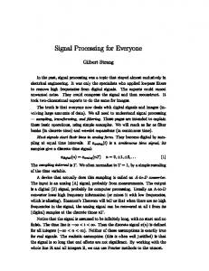
The behavior of SNR with and without interference is illustrated in Fig. 1, where it is assumed that the signal power is equal to the interference power, and that for a single antenna the variance of the independent noise is 20 times (13 dB) greater than the signal power. Note that without interference SNR = 1 is obtained with 20 elements and continues to increase with the number of elements. However, interference of the same average power as the signal limits the achievable SNR regardless of the number of elements used in the array. This example demonstrates the importance of suppressing strong interference, whenever possible, in order to attain the full combining advantage of the array: without interference suppression, the effective aperture of a large array can be significantly reduced. B. Normally Incident Source Fields: Interference Offset from Source If the point interference source is not exactly along the LOS, but still within or near the array beam, then spatial interference canceling techniques can be applied to mitigate the problem, as will be demonstrated in Section IV. The following simple example illustrates the effect of spatial displacement between source and interference on the SNR of the combined signal. Let us suppose that the interfering point source is at an angle θ with respect to the LOS (source still assumed to be at zenith for simplicity), and the weights are chosen to be optimum for the source only, without regard to the interference. The weighted interference contribution from each antenna element picks up an additional phase that depends on the linear distance of that element from some reference point on the array, such as the geometrical center. This is shown in Fig. 2, which illustrates the linear phase gradient picked up by the interference across the array when it is not along the LOS. For very small angles typical of large arrays, the approximation sin(θ) ∼ = θ is valid.

SNR, linear units

10 WITHOUT INTERFERENCE 1

WITH INTERFERENCE (EQUAL TO SIGNAL POWER)

0.1

0.01 1

10 NUMBER OF ANTENNA ELEMENTS, N Fig. 1. SNR as a function of the number of antenna elements, N.

4

100

TOWARDS SIGNAL SOURCE

q

d

TOWARDS INTERFERENCE

d

q

jI (x = -d ) = 2p qd l

jI (x = 0) = 0

jI (x = d ) = 2p qd l

Fig. 2. Source and interference phase geometry across the array.

In Fig. 2, the distance between two elements is taken to be d m, the wavelength is λ, and the additional phase the interference picks up at a distance x from the origin is ϕI (x). If the combining weights are selected to be optimum in the absence of interference, as before, then the signal adds up coherently but the interference components receive a slightly different phase at each antenna element. Assume that N is an odd number, and counting from left to right, we can express the combined output as     N −1 d jεP (t) ∼ y(t) = exp(jωt) N S(t) + B(t)e exp jϕI kd − (N − 1) 2 k=0

+

N

  ni (t) exp − j ϕˆi (t)

(6)

i=1

Writing the exponent in the sum as ϕI (kd − (N − 1)d/2) = 2πθ[−kd + (N − 1)d/2]/λ, the sum inside the brackets can be rewritten in closed form as N −1 k=0

   N −1     πθ(N − 1)d d −2πjkθd = exp exp jϕI kd − (N − 1) exp 2 λ λ k=0



 πN θd sin λ  × ejψ  = πθd sin λ

(7)

2 where ψ is a residual phase. Now the variance of the interference becomes σB sin2 (πN θd/λ)/ sin2 (πθ/λ), which clearly varies with θ, but the signal and noise terms remain as before. Therefore, the SNR now becomes a function of θ and is given by the expression

SNR =

˜ 2] E[|S(t)| 2 2 sin (πN θd/λ) + σn σB N N 2 sin2 (πθd/λ) 2

5

(8)

First, consider the normalized variance due to the combined interference term, as a function of the angle θ. Since the variance of interference is a function of angle, so is the total SNR. The variation of SNR with offset angle is shown in Fig. 3 for the case of 20 elements 10 m apart, a wavelength of 1 cm, and with independent additive noise variance 20 times greater for each element than either the signal or interference power. Note the existence of nulls in the normalized variance at approximately 2.5, 5, and 8 mdeg from the LOS, corresponding to directions where the weighted interference waveforms add up destructively, resulting in complete interference cancellation. In addition, we observe that the larger the angular separation between source and point interference, the smaller the envelope of the combined variance. The total effect of interference plus additive noise on SNR is illustrated in Fig. 4 for the case of 20 antenna elements separated by 10 m, with interference power equal to signal power, and with additive noise power 20 times as great at each element.

NORMALIZED VARIANCE OF N COMBINED ELEMENTS

We observe from Eq. (8) that with θ = 0 degrees and interference power equal to signal power, and with additive noise power 20 times the interference power, the maximum combined SNR with a 20-element array is 0.5. However, as the angle between source and interference increases, the weighted 1.0 0.8

d = 10 m N = 20

0.6 0.4 0.2 0.0 0.000 0.002

0.004

0.006

0.008

0.010 0.012

q, deg Fig. 3. Variance of combined point-source interference, with an offset angle between the source and the interference.

1.2 1.0

SNR

0.8 d = 10 m N = 20

0.6 0.4 0.2 0.0 0.000 0.002

0.004

0.006

0.008

0.010 0.012

q, deg Fig. 4. Total SNR versus offset angle, showing that destructive cancellation effectively eliminates the interference away from the main lobe.

6

interference variance decreases rapidly, until its effect becomes negligible for separations of 10 mdeg or greater. The combined SNR then approaches its noise-dominated value of 1, consistent with the results of Fig. 1. While this is only a 3-dB increase for a 20-element array and the parameters we have selected for illustration purposes, it is clear that the improvement can be much greater for larger arrays: for a 100-element array, the improvement in SNR is 7.8 dB, whereas for a 1000-element array, it exceeds 17 dB. Therefore, elimination or reduction of spatially close interference can result in substantial SNR gain with large arrays. In Sections IV and V, we discuss algorithms that attempt to maximize SNR in the presence of interference and evaluate their performance. C. Extension of Linear Arrays to Simple Two-Dimensional Arrays The results for linear arrays considered above can be extended directly to two-dimensional (2-D) arrays by simply replicating the one-dimensional array orthogonal to its axis, each a specified distance from the previous row, thus creating a two-dimensional array. If an N -dimensional linear array is replicated N times, this results in an N -fold increase in both the signal and interference power collected by the array. More generally, the resulting two-dimensional array may consist of Nx × Ny elements, arranged over the x–y plane as shown in Fig. 5, where the elements are taken to be dx m apart in the x-direction and dy m apart in the y-direction. The phase delays associated with a two-dimensional geometry are slightly complicated due to the additional dimension, but can be attained systematically. Indeed, two-dimensional arrays will be presented in Sections IV and V, where the multiple signal classification (MUSIC) and the eigen algorithms are employed to combine the received signal and to mitigate noise and interferences.

III. Atmospheric Effects: Channel Modeling for the Large Array This section presents the model used in evaluating the combining performance of a very large array. Aside from local noise, as well as external interference from both terrestrial and extra-terrestrial sources (e.g., planets), atmospheric turbulence can significantly alter the received signal phase across the array, thereby degrading combining performance. This is especially problematic at the higher frequencies, i.e., at 17.3 GHz to 32 GHz (Ka-band). Here we consider phase distortions due to turbulence as it moves z y

qa

fa

dx dy

Ny ANTENNAS

Nx ANTENNAS Fig. 5. Two-dimensional array formed by replication of a linear array.

7

x

across the array. This is depicted in Fig. 6 for a uniform linear array of N antennas. The effect of the turbulence is to introduce correlated, temporal signal phase fluctuations. For large arrays and short wavelengths, λ, these fluctuations could severely limit the array’s combining performance. In modeling and simulating the phase fluctuations, we utilize the following signal model: sl (t) = Sl (t) · ejΦl (t) ,

for 1 ≤ l ≤ N

(9)

where Sl (t) is the received (baseband) signal waveform and Φl (t) denotes the total received signal phase, which can be expressed as Φl (t) =

2πld · sin θ + φinst (t) + φprop (t) l l λ

(10)

and d is the distance between elements (Fig. 6). The first term in Eq. (10), (2πld/λ) · sin θ, corresponds to the (ideal) phase associated with a plane wave propagating across the array. The second term, φinst (t), is due to instrumentation effects [1] and l is not addressed here. The third term, φprop (t), is associated with turbulence effects and is the focus of l this section. In evaluating array performance under turbulent atmospheric conditions, we make use of the phase structure function [2]:  2 2 σ∆φ (r) ≡ E |φprop − φprop | ; r ≡ |rl − rk | l k

(11)

where r is the distance between the lth and kth elements and E[·] again denotes time-average expected 2 value. From standard turbulence theory [2], we can express σ∆φ (r) in terms of turbulence parameters as follows:  σ∆φ (r) =

2π λ



 ·C ·h

4/3

·

D


r

(12a)

h

In Eq. (12a), h represents the height of the turbulence (nominally 1 km); C is the turbulence strength parameter (nominally 2.4 × 10−7 m−1/3 ), and D is the (spatially) averaged refractivity:

TURBULENCE PATCH

VELOCITY, V

q

l=1

d

l=N

Fig. 6. N-element array geometry for atmospheric modeling.

8

D(α) =

1 · cos2 θ



1



0

0

1

       2      z−z   − Dχ  z − z  D  α2 + 2(z − z  )α tan θ +  cos θ   · dz · dz (12b)  χ cos θ

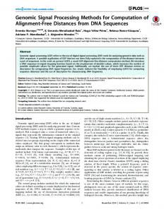
where Dχ (β) = β 2/3 /[1 + (β · h/Γ)2/3 ] is the normalized refractivity structure function and Γ represents 2 the outer scale of the turbulence (nominally 3000 km). In Fig. 7, we present plots of σ∆φ (r) as well as the associated two-element array combining loss as a function of the element separation at two different frequencies: 8.2 GHz (X-band) and 25 GHz. As is seen, the turbulence has a dramatic effect on arraycombining performance at 25 GHz for element separations in excess of 300 m (combining loss >0.5 dB). In modeling these effects, we utilize both the correlation and spectral data derived from turbulence theory [2]. Specifically, the spatial correlation function is given by

2 2 Rφ (r) = 0.5{σ∆φ (∞) − σ∆φ (r)} ≈ 0.5

    

2π  λ   

  2/3  Γ    h 2 − σ (r) ∆φ  cos2 θ   

2 C 2 h8/3

(13)

and the associated spatial phase spectrum is given by 

∞

Sφ (q) = 2

Rφ (r) · cos(2πqr)·dr

(14)

0

where q is the wave number.

2.5

61.5

2.0

55.0

ZENITH

1.5

48.0

1.0

40.0

8.2 GHz (X-BAND) 25 GHz

0.5

27.5

0.0

0.0 101

102 ANTENNA PAIR BASELINE, m Fig. 7. Two-element array combining loss due to turbulence.

9

103

STANDARD DEVIATION OF PHASE DIFFERENCE BETWEEN 2 ARRAY ELEMENTS, deg

COMBINING LOSS FOR 2 ARRAY ELEMENTS DUE TO TURBULENCE, dB

A plot of the spatial correlation function is presented in Fig. 8, corresponding to zenith pointing. As can be seen, the phase fluctuations are highly correlated across the array; however, the phase structure function varies significantly over much shorter scales, as can be inferred from Fig. 8. These scales (10 m–1 km) are typical of large-array inter-element distance [1]. The phase structure function and Sφ (q) are related by

1.0 ZENITH POINTING INDEPENDENT OF l

0.8 Rf(r )/Rf (0)

0.9995 Rf (r)/Rf (0)

0.9

1.0000

0.9990 0.9985 0.9980 0.9975 0.9970

0.7

0

200

400

600

800 1000

ANTENNA SEPARATION, m

0.6

0.5 0.4 0

500

1000

1500

2000

2500

3000

ANTENNA SEPARATION, km Fig. 8. Spatial correlation function.

 2 σ∆φ (r) = 4

∞

  1 − cos(2πqr) · Sφ (q) · dq = 8

0



∞

sin2 (πqr) · Sφ (q) · dq

(15)

0

We approximate Sφ (q) via a fully turbulent model [2] for wave numbers down to q ∼ 1/(10h):  Sφ (q) ∼ 0.016 ·

2π λ

2

C 2 · h · q −8/3 rad2 − m; q > 1/10h

(16)

To derive the temporal phase fluctuation model, we assume a frozen turbulence model wherein the turbulent patches are transported by the wind across the array. Furthermore, identical temporal phase fluctuation spectra, Pφ (f ), are assumed at each antenna site. Based on this model, we can relate Pφ (f ) to the spatial spectrum Sφ (q) via  V 1   f≥  V · Sφ (q)|q=f /V , 10h Pφ (f ) =  1 V   · Sφ (q)| , f< q=1/10h V 10h

(17)

By truncating the spectrum for f < V /(10h) (1 mHz atV = 10 m/s and h = 1 km), we are ignoring very low frequency components that are constant over the time scales of interest. Discrete-time realizations of the fluctuating phase at each antenna output are first generated by digitally filtering independent, white, zero-mean, Gaussian inputs, as depicted in Fig. 9. The digital filter response H(f ) is most conveniently generated in the frequency domain via the fast Fourier transform (FFT): 10

SCALE FOR UNIT OUTPUT VARIANCE (t ) H( ) = WHITE GAUSSAIN SEQUENCE (zero-mean/ unit variance)

f (t )

Pf ( )

= antenna index

(t ) k (t ) = 0; k Fig. 9. Generating independent phase correlation functions.

 H(k) =

  Pφ (f )

H(2N − k) = H(k),

, f =k·Fs /2N

1≤k≤N

0≤k≤N

        

(18)

where Fs = sample rate > 4 · V /h. A sample digital filter response is depicted in Fig. 10; a sample independent realization is depicted in Fig. 11. The next step in generating phase realizations is to build in the spatial correlation properties. This is done by first forming the spatial correlation matrix R from the spatial correlation function, i.e., [R]k ≡ Rφ ( d − kd)

(19)

√ and then constructing the square root of this matrix, i.e., R. The desired spatially correlated phase realizations are then created by appropriately combining the independent phase realizations, as depicted in Fig. 12. In this manner, the corresponding output phase data φprop (t) are guaranteed to have the  correct temporal and spatial statistics. Sample realizations are depicted in Fig. 13, corresponding to the following parameters: N = 20 antennas d = 500 m frequency = 25 GHz (Ka-band) vertical incidence, θ = 0 deg Fs = 100 V/h = 1 Hz turbulence parameters: V = 10 m/s h = 1 km Γ = 3000 km Fs = 100 V /h = 1 Hz As is seen in Fig. 13, although the phase fluctuations apparently have an extremely high degree of correlation, the corresponding phase difference data obey the modeled spatial structure function. 11

1.0 0.8 0.6

(b)

0.8

V = 10 m/s h = 1 km Fs = 100 V/h = 1 Hz

h (t )

H (f )

1.0

(a)

0.4

0.6 0.4

f -4/3 0.2

0.2

0.0

0.0 0

5

10

15

20

25

0

200

f, mHz

400 t, s

Fig. 10. Typical digital filter response: (a) frequency filter response magnitude and (b) filter impulse response.

2

f (t ), rad

1 0 -1 0

500

1000

1500

2000

t, s Fig. 11. Sample phase realization.

INDEPENDENT PHASE GENERATOR

f1 (t )

f prop(t )

f prop(t )

f prop(t )

1

1

R

1

f prop (t )

f N (t )

N

f prop(t ) 1 Fig. 12. Generation of spatially correlated phase realizations.

The computer model presented herein accurately models the phase structure function computed from pairs of elements. In particular it is shown that at the higher frequencies (25 GHz and above), significant combining loss (0.5 dB or more) can occur for element baselines in excess of 300 m due to atmospheric turbulence. However, phase realizations generated by the computer model reveal that these effects occur at very low frequencies compared to the signal bandwidths of interest. Thus, they potentially can be compensated for via smart adaptive array processing. Nevertheless, these effects must be taken into account in developing combining algorithms for large-array antennas.

IV. MUSIC Algorithm and Beam Forming Spatially correlated interference poses challenges to the array-combining problem. To address the issues of identifying the intended and interference signals, and, furthermore, to suppress these interference

12

f0prop(t ), rad f1prop(t ), rad f2prop(t ), rad f3prop(t ), rad f4prop(t ), rad f5prop(t ), rad

15 0 -15 15 0 -15 15 0 -15 15 0 -15 15 0 -15 15 0 -15

f0prop(t ) - f1prop(t )

1.5 0 -1.5 1.5 0 -1.5 1.5 0 -1.5 1.5 0 -1.5 1.5 0 -1.5

0

1000

2000 3000

4000 5000

f0prop(t ) - f2prop(t ) f0prop(t ) - f3prop(t )

sDf(D) = 39/40 deg (theory/sample) sDf(2D) = 56/52 deg (theory/sample) sDf(3D) = 69/64 deg (theory/sample)

f0prop(t ) - f4prop(t ) f0prop(t ) - f5prop(t ) 0

1000

2000 3000

t, s

sDf(4D) = 78/77 deg (theory/sample) sDf(5D) = 86/79 deg (theory/sample)

4000 5000

t, s

Fig. 13. Correlated phase realizations.

signals, direction-finding algorithms and interference-suppression techniques are combined and studied. In particular, high-resolution direction-finding algorithms are focused on in this section. They do not have the problem associated with most of the conventional Fourier transform-based approaches, which are inherently limited by relatively high side lobe and, therefore, lower resolution. High-resolution eigenstructure-based methods incorporate both amplitude and phase information to achieve high-resolution angle-of-arrival (AOA) estimates for multiple incident sources. These techniques stem from Schmidt’s multiple emitter location and signal parameter estimation (MUSIC) algorithm [3]. To illustrate the essential features of the MUSIC algorithm, we consider an N -element array (assuming complex baseband data format) with up to L different signal sources incident upon the array at AOAs θ1 , · · · , θL . Define the array manifold, A(θ), which is an N × L matrix comprising the vectors of array responses, a(θi ), modeled or measured during calibration: A(θ) = [a(θ1 ) a(θ2 ) · · · a(θL )]. Furthermore, define S(t) to be the L × 1 vector of radiated signals incident upon the array at time t, and n(t) to be the N × 1 vector of receiver measurement noise. It is assumed in the following that the components of n(t) are zero-mean and independent noises with variance σn2 . The received array signal vector can then be written as X(t) = A(θ) · S(t) + n(t)

(20)

The direction-finding problem is to estimate the unknown angles of arrival, θ1 , · · · , θL , given X(t), t = 1, · · · , M , where M is the number of received signal samples. Given that the array response vectors are orthogonal to the eigenvectors spanning the noise subspace [3], MUSIC uses the following procedure for estimating the AOAs: first form the sample covariance matrix R and perform an eigen-decomposition for Hermitian matrices, i.e.,

R=

M 1 X(t)X H (t) = V · Λ · V H M t=1

13

(21)

where H denotes the conjugate transpose operation, Λ = diag(λ1 , λ2 , · · · , λN ), with the eigenvalues satisfying λ1 ≥ λ2 ≥ · · · ≥ λN , and V = [ v1 v2 · · · vN ] are the corresponding orthonormal eigenvectors of R. The unitary matrix of eigenvectors V can be decomposed further as V = [Vs Vn ], where the columns of Vs comprise the eigenvectors corresponding to the L largest eigenvalues of R (the signal subspace), and where Vn contains the remaining (noise) eigenvectors. Next the inverse MUSIC spectrum, F (θi ), is formed via F (θi ) ≡

1 VnH

· a(θi )

(22)

2

Since the array response vectors a(θi ) are orthogonal to the eigenvectors spanning the noise subspace Vn , ! !2 it can be seen that the AOA estimates will occur at those θi ’s that satisfy the equation !VnH · a(θi )! = 0, arg max yielding the AOA estimate θˆ = {F (θi )}. The method can be readily extended to two-dimensional θ1 arrays, as illustrated in the following. As an example, Fig. 14 presents the results of applying MUSIC to a one-dimensional array configuration (10-element uniform linear array with half-wavelength spacing) with an incident signal and three interference plane wave components (to emulate planetary interference). The power in all signal and interference components is assumed to be equal in this example, and the SNR per element is −15 dB. Figure 14(b) is the array response without adaptive interference cancellation. The three vertical straight lines indicate the location of the interfering sources. The MUSIC algorithm is first used to identify the desired signal, impinging on axis, followed by identification of the three interference signals. Once these AOAs have been identified, an interference cancellation technique, such as the linear constrained minimum-variance (LCMV) algorithm or the side lobe canceler, can be used to suppress the undesired interference sources. The antenna pattern presented in Fig. 14(a) is an example of the result from using LCMV. This approach can be further extended to form a continuous area of nulls in the spatial domain. In Fig. 15, a large planetary interference source has been modeled as a series of clustered distributed sources (again with the same power in the signal and interference components and approximately −15 dB 40 (a) GAIN, dB

30 20 10 0 40 GAIN, dB

(b) 30 20 10 0 -1.0 -0.8

-0.6

-0.4

-0.2

0.0

0.2

0.4

0.6

0.8

u, sines Fig. 14. MUSIC and adaptive cancellation: (a) with three-null cancellation and (b) without cancellation.

14

1.0

40 (a) GAIN, dB

30 20 10 0 40 (b) GAIN, dB

30 20 10 0 -1.0 -0.8

-0.6

-0.4

-0.2

0.0

0.2

0.4

0.6

0.8

1.0

u, sines Fig. 15. MUSIC and zone cancellation: (a) with multiple-null (zone) cancellation and (b) without cancellation.

SNR per element). Provided the number of antenna elements in the array has a sufficient number of degrees of freedom, typically on the order of 2 to 3 times that of the number of interferers, the adaptive cancellation technique, together with MUSIC, can be very effective for mitigating planetary interference. In such cases, large arrays can provide significant advantages over single-aperture antennas for multibeam applications, such as improved SNR through suppression of planetary noise, together with robust operation and improved availability. When using the MUSIC algorithm, it is important to differentiate between the intended signal and spatially correlated interference signals. A JPL-developed generalized pre-processor algorithm [8,9] can be used to identify the intended signal and has been incorporated into the simulations. The concept presented there originated from the phase estimation problem under conditions of very low SNR characteristic of distant spacecraft, emergency-mode communications, and reception of turbo-coded signals where symbol SNRs of −6 dB are routinely encountered [10]. This technique also can provide significantly improved phase estimates for the individual elements of a large antenna array. As an example of operation with a 20-element linear array, Fig. 16 shows the MUSIC pseudo-spectrum of simulated spacecraft and planetary sources. Figure 17 shows the corresponding results after the preprocessor has been turned on. The incorporation of low SNR generalized pre-processor structures for coded telemetry clearly enables greatly enhanced identification of spacecraft signals in the presence of spatially overlapping interference when using the MUSIC algorithm. The approach of combining high-resolution direction finding using MUSIC and interference cancellation using beam forming can be extended from a one-dimensional to a two-dimensional planar array. Figure 18 illustrates the two-dimensional inverse MUSIC spectrum of an 8-by-8 square planar array (half-wavelength vertical and horizontal spacing between elements). The signal of interest arrives from (θ = 50 deg, φ = 0 deg), and the interfering signal arrives from (θ = 10 deg, φ = 0 deg), where θ is the angle from the normal to the array and φ is the corresponding azimuthal angle. These two signals are of equal power (under noiseless conditions) and can be readily identified in the two-dimensional inverse MUSIC spectrum. Figure 19 is a regional top view of the inverse spectrum where the two local peaks are clearly formed at the two impinging directions. 15

25

MUSIC SPECTRUM, dB

20 15

DESIRED SPACECRAFT SIGNAL

INTERFERENCE

10 5 0 -5 -10 -15 -100 -80 -60 -40 -20

0

20

40

60

80 100

AOA, deg Fig. 16. Pseudo-spectrum of simulated spacecraft and planetary source. 15

MUSIC SPECTRUM, dB

10

DESIRED SPACECRAFT SIGNAL

5

0 -5 -10 -15 -100 -80 -60 -40 -20

0

20

40

60

80 100

AOA, deg Fig. 17. MUSIC plus pre-processor.

Given the angle of arrival estimates, two-dimensional adaptive beam-forming techniques can be carried out to derive the optimum combining weights for the planar array. The two-dimensional antenna pattern with these weights is plotted in Fig. 20. In this example, the signal of interest comes from (θ = 50 deg, φ = 50 deg), and four interfering signals impinge from (θ = 20 deg, φ = 20 deg), (θ = 20 deg, φ = 15 deg), (θ = 15 deg, φ = 20 deg), and (θ = 15 deg, φ = 15 deg). The four point sources form a square, which models a planar interfering source. The beam-forming algorithm is able to null out the interfering sources, as seen in Fig. 20 as well as in the regional top view of Fig. 21. The original beam pattern of the planar array is shaped to enhance the signal of interest while simultaneously nulling the interfering signals. The communications performance of the MUSIC algorithm with beam forming can be assessed in terms of the combining loss associated with the output signal of the array, that is, the loss compared to a perfectly phased array of antennas. The results using this method are displayed in Fig. 22. Only signal plus receiver noise is considered in this example, with no additional interference signals. The number of symbols within a block ranges from 5000 to 60,000 for each process. The combined output symbol SNR is fixed at −7 dB, and the received symbol SNR at each receiver is −(7+10 log10 N ) dB. Thus,

16

2-D PSEUDO-SPECTRUM, dB

-11 -12 -13 -14 -15 -16 -17 -18 -19 100 50 0 q, deg

-50

60

40 20

-100

80

100

f, deg

0

Fig. 18. 2-D MUSIC pseudo-spectrum (8-by-8 array), signal from (q = 50 deg, f = 0 deg) and the interfering signal from (q = 10 deg, f = 0 deg). 90 -12

80 70

-13

60

q, deg

-14 50 40

-15

30

-16

20 -17 10 -18

0 0

10

20

30

40

50

60

70

80

90

f, deg Fig. 19. Regional top view of MUSIC pseudo-spectrum (8-by-8 array), signal from (q = 50 deg, f = 0 deg) and the interfering signal from (q = 10 deg, f = 0 deg).

the larger the array size, the smaller the received symbol SNR at each receiver. This accounts for the relatively large combining loss for the larger arrays. It can be seen that, when the number of symbols exceeds 40,000 (where log10 (40, 000) = 4.6), less than 0.5-dB combining loss can be achieved with arrays of 128 or fewer elements.

V. Eigen-Based Combining Algorithms Traditional eigen-based combining algorithms (see a detailed survey in [4]) for large-array antennas require forming the covariance matrix of the observables between the array elements and solving an 17

PLANAR ANTENNA PATTERN (LINEAR)

90 80 70 60 50 40 30 20 10 0 100 80

100 60

50 40

0

f, deg

20

-50

0

-100

q, deg

Fig. 20. Antenna pattern with adaptive beam-forming techniques (8-by-8 array), signal from (q = 50 deg, f = 50 deg) and interference from (q = 20 deg, f = 20 deg), (q = 20 deg, f = 15 deg), (q = 15 deg, f = 20 deg), and (q = 15 deg, f = 15 deg).

90

80

80 70 70 60 60 f, deg

50 50 40 40 30

30

20

20

10

10 0 0

10

20

30

40

50

60

70

80

90

q, deg Fig. 21. Top view of the adaptive beam-forming pattern (8-by-8 array), signal from (q = 50 deg, f = 50 deg) and interference from (q = 20 deg, f = 20 deg), (q = 20 deg, f = 15 deg), (q = 15 deg, f = 20 deg), and (q = 15 deg, f = 15 deg).

eigenvalue problem. While they yield the optimal combining weights, these methods require a signal correlator, which for a large-sized array can be time consuming and expensive. In this section, we investigate two combining approaches: one is designed to reduce the number of operations required to attain the optimal weight by means of iteration and the other is designed to find the optimal weight that mitigates strong interferences and noise. Mathematical frameworks, numerical algorithms, and computer simulations for both techniques will be presented. 18

2.5 8 ANTENNAS 16 ANTENNAS 32 ANTENNAS 64 ANTENNAS 128 ANTENNAS

COMBINING LOSS, dB

2.0

1.5

1.0

0.5

0.0 3.6

3.8

4.0

4.2

4.4

4.6

4.8

5.0

NUMBER OF SYMBOLS (log10(N )) Fig. 22. Combining performance of MUSIC with beam forming, as a function of the number of symbols

The array model is similar to that discussed in Section II, that is, there are N identical receivers in a linear array separated by the same distance. We denote by ϕi (t) the phase angle between the spacecraft and the ith antenna. as well as K other point-source " Each antenna receives a signal S(t) from the spacecraft # P interferences B1 (t) exp(j(ϕi (t) + εP (t))), B (t) exp(j(ϕ (t) + ε (t))), · · · , BK (t) exp(j(ϕi (t) + εP 2 i 1 2 K (t))) , each of which is directly behind the spacecraft and differs in phase by εP k (t) for some k = 1, 2, · · · , K. N Independent white Gaussian noise waveforms, {ni (t)}i=1 , also are added to the observables. Furthermore, we assume that the point-source interference and the internally generated receiver noise are uncorrelated. Based on this model, the ith antenna generates the IF waveform

Xi (t) = si (t) +

K

bi (k) + ni (t)

(23)

k=1

where si (t) = S(t) exp(jϕi (t)) and bi (k) = Bk (t) exp(j(ϕi (t) + εP k (t))). We remark here that the algorithms in this section belong to a class of blind combining techniques and that no spatial information of N the spacecraft and the ground receivers is needed. The observables {Xi (t)}i=1 generated in Eq. (23) are $K merely for simulation purposes. By denoting the undesired components by zi (t) ≡ k=1 bi (k) + ni (t), Eq. (23) can be rewritten as Xi (t) = si (t) + zi (t)

(24)

N

Our goal is to find an optimal set of weights {wi }i=1 so that the combined output signal

Y (t) =

N

w ¯i Xi (t)

(25)

i=1

achieves certain objectives. Particular objectives considered in this section include (1) maximizing the combined output power (MCOP) and (2) maximizing the combined output signal-to-interference plus noise ratio (MCOSINR). Next, we will discuss the mathematical frameworks for these objectives as well as the details of our proposed approaches. 19

A. Maximizing the Combined Output Power (MCOP) As its name indicates, the MCOP algorithm is designed to find a normalized set of weight that maximizes the combined time-average output signal power, which we define as E[||Y (t)||2 ], where E[·] again denotes the time-average expected value operator. It can be shown easily that the combined output signal power can be expressed in the quadratic form of the covariance matrix, i.e., %   N & 2  M     1 E[||Y (t)||2 ] = E 

H w ¯i Xi (t) = w Xi (m)XiH (m) w

=w

H Rw

M

(26)

m=1

i=1

Taking advantage of the eigen decomposition of the covariance matrix R defined in Eq. (21), any arbitrary set of unit weight w

can be written as

w

=

N

αi vi = V α

(27)

i=1

where α

= [α1 , α2 , · · · , αN ]T and

$N i=1

|αi |2 = 1.

Putting the combined output power, Eq. (26), in normalized form, we have N    2 E Y (t) = (V α

)H V ΛV H (V α

) = α

H Λ α= λi |αi |2 ≤ λ1

(28)

i=1

Therefore, the weight that yields the largest combined output power is the eigenvector that corresponds to the largest eigenvalue. Traditional procedures for finding the dominant eigenvector include the following: (1) Form the covariance matrix R. (2) Solve the eigen problem R v = λ v and sort the eigenvalues λ1 ≥ λ2 ≥ · · · ≥ λN . (3) Set w

opt = v1 . Note that the above approach solves for all eigenvectors, while it uses only the dominant one. Therefore, a more efficient technique is needed, which turns out to be a well-known numerical algorithm called the power method [5]. The power method finds iteratively and solely the dominant eigenvector and is implemented as follows: (1) Form the covariance matrix R. √ (2) Start with w

(0) = [1, · · · , 1]T / N and compute successively w

(k) = Rw

(k−1) /||Rw

(k−1) ||. (3) Set w

opt = w

(k) . Note that while it eliminates many of the unnecessary computations of non-dominant eigenvectors, the power method requires the formation of the covariance matrix R. As a result, the total number of floatingpoint operations is N (N + 1)M/2 + N 2 I, where again N is the number of antennas, M is the number of signal samples within a received block, and I is the number of iterations. To reduce further the number of floating-point operations and to remove the requirement for forming the covariance matrix, we propose the following algorithm, which we call the matrix-free power method: 20

√ (1) Start with an initial guess w

(0) = [1, · · · , 1]T / N . (2) Compute successively w

(k) = u(k) /|| u(k) ||, where (k)

uj

  = E Xj (t)Y¯ (t)

Y (t) =

N

(k−1) w ¯i Xi (t)

          

(29)

i=1

(3) Set w

opt = w

(k) . (k)

With simple algebraic manipulations, one can see that uj in Eq. (29) is exactly Rw

(k−1) . The number of floating-point operations is reduced to N · M · I. The convergence of the power method is dictated by the separation of the signal power to the noise power and the number of iterations is bounded, in the worst-case scenario, by N . Moreover, the number of iterations may be large for the first block of symbols, but, in most cases, I