canopy upstream and downstream from a single fence, and found that the ... of repeating fences set within a simulated wheat canopy to better understand the.
LARGE-EDDY SIMULATION OF WINDBREAK FLOW EDWARD G. PATTON∗ and ROGER H. SHAW Department of Land, Air and Water Resources, University of California, Davis, U.S.A.
MURRAY J. JUDD The Horticultural and Food Research Institute of New Zealand Ltd., Kerikeri, New Zealand
MICHAEL R. RAUPACH CSIRO Centre for Environmental Mechanics, Canberra, Australia
(Received in final form, 23 January, 1998)
Abstract. A large-eddy simulation has been performed of turbulent flow around multiple windbreaks set within a wheat canopy under neutral stability conditions. The simulation is validated against a wind tunnel data set taken under similar conditions. Velocity profiles and second-order statistics are presented and compared to those found in the wind tunnel. From the numerical simulation, we discuss spatial distributions of instantaneous velocity fields and pressure statistics, which are important and telling features of the flow that are difficult to measure experimentally. We present a discussion of the momentum balance at various locations with respect to the windbreak, and similarly, we introduce the budget of a passive scalar. These discussions show the importance of the terms in each budget equation as they vary upstream and downstream of the windbreak. Keywords: Canopy, Large-eddy simulation, Windbreak, Wind tunnel
1. Introduction Windbreaks have been used for an undocumented period of time to provide protection for crops, to reduce soil erosion, and to control snow drift, and are frequently installed in multiple arrays. Scientists have investigated the influence of such obstacles for decades, yet their aerodynamic performance is not well understood, nor are their overall effects on crop production. An early review of windbreaks and shelter belts is provided by van Eimern et al. (1964). Summarizing the aerodynamics of shelter, they point to permeability as the main factor in regard to downstream distribution of wind speed, and identify a permeability of 40 to 50% as having the most extensive wind speed reduction. In this case, the minimum windspeed is found four to six shelter heights in the lee of the break. They say that relative wind reduction is rather insensitive to the magnitude of the wind but that the surface roughness and atmospheric stability are important. ∗ Current affiliation: University of Minnesota, Department of Soil, Water, and Climate, St. Paul,
Minnesota, U.S.A. 55108. Corresponding address: National Center for Atmospheric Research, P. O. Box 3000, Boulder, CO, U.S.A. 80307-3000. Boundary-Layer Meteorology 87: 275–306, 1998. © 1998 Kluwer Academic Publishers. Printed in the Netherlands.
276
E. G. PATTON ET AL.
It was realized that the upstream flow has a large effect on the protection provided by the presence of a break. Argent (1992) investigated the effects of a plant canopy upstream and downstream from a single fence, and found that the presence of a canopy upstream significantly reduced the size of the protection zone. Iqbal et al. (1977) and McAneney and Judd (1991) discussed the effects of multiple windbreaks and of increased upstream roughness. Papesch (1992) performed wind tunnel experiments in an attempt to find the barrier spacing and fence porosity that provided the best wind speed reduction at ground level. It was found that increased roughness increased the turbulence intensity of the approach flow, and resulted in a smaller region of protection as high momentum fluid penetrated downwards more rapidly. Recently, Judd et al. (1996) performed a wind tunnel investigation of repeating fences set within a simulated wheat canopy to better understand the underlying physics, and to design optimized configurations for crop protection. Few attempts have been made to numerically simulate the complex flow field associated with windbreaks. Those studies in the literature solve the Reynolds averaged equations of motion using various orders of closure, and different boundary conditions and forcings (Durst and Rastogi, 1980; Hagen et al., 1981; Wilson, 1985; Liston et al., 1993). Durst and Rastogi (1980) and Liston et al. (1993) used a variant of a k-� model to simulate a solid fence, which is decidedly different from the porous case discussed in Hagen et al. (1981). Wilson (1985) improved upon Hagen et al.’s (1981) simulation by properly parameterizing the drag imposed by the fence, and determining the best choice of closure schemes. Most recently, Wang and Takle (1995) presented numerical solutions to the flow around a single fence using a closure similar to Yamada (1982). They show detailed two-dimensional (x, z) contours of wind speed, static pressure, and turbulent kinetic energy ahead of and in the lee of the break. More than two decades ago, Deardorff (1970) proposed a numerical technique that would retain most of the essential physics, but would eliminate the need to Reynolds average the flow field. He proposed that, by using a three-dimensional grid network with sufficient resolution, the larger, energy containing scales of motion would be resolved, with only motions smaller than the grid dimensions needing to be parameterized. He suggested that if those subgrid-scale motions fell within the inertial sub-range, they would not contribute significantly to the fluxes of heat and momentum but, rather, would act mainly to dissipate energy. This technique has become known as large-eddy simulation (LES), and has been used extensively in geophysical and engineering flows. Here, we present a large-eddy simulation of the separated flow associated with surface mounted porous obstacles set within a plant canopy under neutral stability conditions. Because end boundary conditions in LES are necessarily periodic, we simulate what is essentially an infinite set of equally spaced windbreaks. We note again that multiple windbreak arrays are employed extensively in agricultural and horticultural settings. We show a detailed comparison with a wind tunnel experiment (Judd et al., 1996) of average flow fields and second-order statistics. We also
LES OF WINDBREAK FLOW
277
present budgets of momentum and of a passive scalar that provide insight into the mechanisms responsible for the complex flow fields that result from interactions with a porous shelter.
2. The Large-Eddy Simulation 2.1. T HE
EQUATIONS
We employ the large-eddy simulation (LES) described by Moeng (1984) and Moeng and Wyngaard (1988). The LES technique integrates a set of three-dimensional, filtered Navier-Stokes equations under the Boussinesq approximation. We include additional terms representing drag by the canopy elements, and similarly, the drag imposed by the windbreak. Using index notation, the filtered equations are: ∂ui = 0, ∂xi
(1)
∂ui ∂ui 1 ∂P ∂π ∂τij =− − − + Fi , + uj ∂t ∂xj ρ◦ ∂xi ∂xi ∂xj
(2)
where ui is the resolvable scale velocity in the xi direction, τij is the trace-free subgrid-scale (SGS) stress defined as τij = (ui uj − u¯ i u¯ j ) −
δij (uk uk − u¯ k u¯ k ) 3
(3)
where ui is the total velocity defined as ui = u¯ i + u0i (total = resolved + subgrid). Here, i, j, k = 1, 2, or 3 representing the streamwise x, spanwise y, or vertical z directions. The first term on the right hand side of Equation (2) represents a prescribed large-scale pressure gradient, which is uniform throughout the domain and is aligned in the x-direction (i.e., ∂P /∂xi = 0 for i = 2, 3). A constant integrated mass flow across the upwind y, z plane is maintained by an adjustment of this term at each timestep. The total pressure ( p) can be decomposed as p = P + p + p0 ,
(4)
where P represents the resolved-scale domain-averaged pressure, p is the deviation of the resolved-scale pressure from this domain average, and p 0 is an unresolved subgrid-scale perturbation. The quantity π is defined as π=
p 1 + (uk uk − u¯ k u¯ k ) ρ◦ 3
(5)
278
E. G. PATTON ET AL.
and represents the sum of the resolved-scale kinematic pressure and the contribution from normal SGS stresses. Fi is the drag imposed by either the wheat canopy or the windbreak in the xi direction. In the code, the non-linear advection terms are written in rotational form (i.e., the sum of the cross product of velocity and vorticity and the gradient of kinetic energy), but are presented here in their more classical form for clarity. We have neglected the Coriolis force, as it has little bearing on the scales of motion in which we are interested (nor would it under field conditions). Molecular diffusion has also been neglected except for its influence in energy dissipation, which will be discussed later. The gravitational term in the vertical momentum equation has also been eliminated since we are simulating a neutral stability situation. We include a conservation equation for a passive scalar in addition to the momentum equations. The wheat canopy is treated as a source of the scalar. The equation for the scalar is ∂B ∂τiB ∂B =− + S, + ui ∂t ∂xi ∂xi
(6)
where B represents the resolved portion of any passive scalar, τiB is the SGS flux of the scalar, and S is the volumetric source density which will be defined later. 2.2. S UBGRID - SCALE
CLOSURE
The momentum and scalar equations contain terms for the SGS fluxes, which are determined from the resolved-scale variables and the SGS kinetic energy. Following Deardorff (1980), we integrate a prognostic equation for the SGS kinetic energy e0 , where e0 = (uk uk − u¯ k u¯ k )/2: ∂e0 ∂e0 ∂ u¯ i e0 ∂[u0i (e0 + p 0 /ρ◦ )] = −τij − − 2 − �, + ui ∂t ∂xi ∂xj ∂xi τ
(7)
where τ is a time scale for the drag and will be defined in Equation (15), and � is the viscous dissipation rate. The SGS fluxes are determined from the resolved-scale variables by � τij = −KM
τiB = −KB
∂ui ∂uj + ∂xj ∂xi
∂B , ∂xi
� ,
(8)
(9)
where KM and KB are SGS eddy coefficients for momentum and the passive scalar.
LES OF WINDBREAK FLOW
279
In order to solve Equation (7), the second and last terms on the right hand side need to be parameterized. For the first of these we make an assumption of downgradient diffusion for subgrid scales. The parameterization is written in the form u0i (e0 + p 0 /ρ◦ ) = −2KM
∂e0 , ∂xi
(10)
For the dissipation term in Equation (7), we make use of the Kolmogorov hypothesis by writing �=
c� (e0 )3/2 , l
(11)
where the value of c� is equal to 0.93 according to Moeng and Wyngaard (1988) and l is a representative length scale which, for this problem, is defined in Equation (12). The second to last term in Equation (7) represents the removal of SGS kinetic energy by wake motions generated by the drag elements as described by Shaw and Schumann (1992). All scales of motion larger than the grid are resolved, and the effects of the drag elements on the resolved velocities are explicitly included in Equation (2). Shaw and Seginer (1985) suggested that an energy transfer occurs between both the time mean flow and the large scale turbulence to the wake scale. We have included this term in Equation (7) under the assumption that wake motions generated by the drag are smaller scale than those responsible for the majority of the SGS energy, and therefore that wake scale motions make no contribution to the turbulent kinetic energy; they are assumed to be small enough in scale that they dissipate rapidly. The length scale l has been defined for this problem as �1/3 � 3 3 , (12) dx × dy × dz l= 2 2 where dx, dy, and dz are the grid dimensions, and the constants ( 32 ) arise due to the wave-cutoff filtering process which will be discussed later. Since we are simulating a neutral case, there has been no allowance for stability dependence. We have also not allowed l to vary as the wall is approached. The eddy diffusivities for momentum and the passive scalar are proportional to 1/2 the product of the SGS length scale ( l) and a SGS velocity scale (e0 ). KM and KB are written as KM = ck l(e0 )1/2
(13)
and KB = 3KM .
(14)
280
E. G. PATTON ET AL.
where ck = 0.1. The value of ck and the other constants used in Equations (10), (11), and (14) are entirely empirical (Deardorff, 1980; Moeng, 1984), however, these constants should not drastically affect the simulation since they only impact SGS processes. 2.3. N UMERICAL
METHODS
We use a pseudospectral differencing technique to estimate horizontal derivatives. To approximate vertical derivatives for the velocity fields, we use a second-order centered-in-space finite difference scheme, while for the scalar field, we use the monotone scheme described in Koren (1993). Taking the divergence of Equation (2) forms a Poisson equation for the quantity π which we use to force incompressibility and to solve for pressure (p). Following Sullivan et al. (1996), we use a third-order Runge-Kutta scheme to advance in time. We impose a staggered grid system in the vertical and a non-staggered grid in the horizontal. The variables w and e0 are located at the ground surface, and the variables u, v, B, and p are located one-half grid point above the surface. The domain is comprised of 96×96×30 grid points in the x, y, z directions, with grid spacings dx, dy, dz which are equal and constant through the domain at 0.02 m in this numerical representation of the conditions in the wind tunnel. The wind break, which is eight grid points tall, is positioned normal to the mean flow, and is located at grid point sixteen in the x-direction spanning the entire y-direction. The wheat canopy is spatially homogeneous (except where the windbreak resides) and occupies the lowest three grid points. While this provides a rather poor resolution of the wheat canopy, we consider it a sufficient representation of an underlying crop for the purposes at hand. The wind speed integrated across the upwind y, z plane is fixed by a uniform streamwise pressure gradient at 6 m s−1 , but in order to perform comparisons with the wind tunnel data, we scale the velocities to match each other. According to the Courant criterion, based on the y, z integrated velocity and a grid dimension of 0.02 m, the timestep is set at 1.0 × 10⁻³ s. While the imposed pressure gradient is unusually large and its repercussions uncertain, alternatives are either computationally very expensive (nesting our fine grid domain into a larger, coarse grid network) or unacceptably intrusive (imposing a large SGS momentum flux at the upper boundary). Periodic boundary conditions are imposed in the horizontal directions, thus the windbreak repeats itself every twelve windbreak heights in the streamwise direction. This contrasts with the wind tunnel simulation which was limited to three windbreaks with only the center one used for measurement purposes. The upper boundary is set as a frictionless rigid lid, with zero flux of mass, momentum, SGS energy, and the scalar. No-slip conditions are imposed at the ground surface, where the stress is calculated from a prescribed surface roughness length and the velocity at one-half grid point above the surface. We use this condition at the surface with
LES OF WINDBREAK FLOW
281
the understanding that the important sink for momentum is in the upper layers of the wheat canopy, and that what happens at the soil surface is much less important. Arnal and Friedrich (1993) investigated the influence of the spanwise dimensions on the predicted mean flow characteristics for separated flows over a backward-facing step. They found for a spanwise dimension of eight step heights or more, periodic boundary conditions could be used in that direction without influencing the predicted location of re-attachment. In our simulation we use a spanwise dimension equaling twelve fence heights, which more than adequately satisfies this requirement. Following Moeng and Wyngaard (1988), we use a wave-cutoff filter in the horizontal directions to separate resolved and SGS motions, and to eliminate aliasing problems. In Fourier space, we truncate the highest one-third of the resolved modes. A result of such filtering can be seen in Equation (12) where we must define a length scale that is larger than the grid dimensions. To calculate mean fields and statistics for the LES data, we average over all y for a given x, z position. With only 96 grid points in the y-direction, we perform this y averaging for all x, z grid points, and then average over 10,000 timesteps in order to ensure stable statistics. The choice of 10,000 timesteps is made to average over at least four large-eddy turnover times, complementing the y averaging process. We introduce the notation h iy,t to denote such an averaging process, and 00 to represent a departure from that average. The 10,000 timestep simulation from which we calculate the averaged fields took nearly 130 CPU hours on a Cray J920, which translates to 10 s of wind tunnel time, a ratio of 46,800 to 1, computational time to simulated wind tunnel time. Scaling to the outside world, for 5 m tall shelters separated by distances of 60 m, and with a mean wind speed of 3 m s−1 , the 10,000 timesteps scale to about 667 s or around 11 minutes of real time. 2.4. D ESCRIPTION
OF SURFACE DRAG ELEMENTS
The drag imposed by either the wheat canopy or the windbreak is written as Fi = −Cd aV ui = −
ui , τ
(15)
where Cd is an isotropic element drag coefficient, a is a leaf area density (the one-sided leaf area per unit volume), and V represents the current scalar speed (ui ui )1/2 . The wheat canopy is defined as a horizontally and vertically uniform spatial distribution of drag elements with a leaf area density of 10.6 m−1 and a drag coefficient of 0.4725 to match the wind tunnel experiment. In the wind tunnel experiment (Judd et al., 1996), the aerodynamic density of the fence was expressed in terms of a pressure coefficient k, which is defined according to δp = kρU 2 /2, where δp is the measured pressure drop across the fence. Assuming that the aerodynamic drag of the windbreak approximately balances the
282
E. G. PATTON ET AL.
pressure drop, and for a spatially continuous distribution of windbreak material, following Wilson (1985), we may write Z (16) k = 2 Cd adx. where Cd and a refer to the drag coefficient and area density of the components of the windbreak. Since our windbreak occupies a single grid interval in the xdirection, the discrete equivalent to this expression is simply k = 2Cd a dx.
(17)
With dx being the grid spacing. It is noted that the leaf area density and the drag coefficient are inseparable in the expression for the drag force, so the only factor of importance is their product. For simplicity, the source (S) of the passive scalar is considered to be independent of time and horizontally homogeneous. It is distributed vertically through the wheat canopy in a manner to approximate the absorption of solar radiation as would be the case for water vapor released from leaves during transpiration. Allowing solar radiation to be depleted according to the exponential of the downward cumulative leaf area index, which in this case of uniform element area density is a linear function of height, we obtain a source strength which decreases exponentially with depth. We chose an extinction coefficient of 0.6 but, because of the sparse nature of the canopy in question, the source strength diminishes by only 26% from top to bottom of the canopy. The windbreak makes no contribution to the scalar concentration.
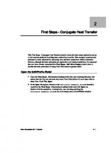
3. The Wind Tunnel Experiment The wind tunnel experiment is fully described by Judd et al. (1996) and only the important details of the experiment will be presented here. The open-return blower tunnel has a working length of 10.1 m, a width of 1.8 m, and an adjustable roof of height approximately 0.7 m to eliminate longitudinal pressure gradients. A schematic of the tunnel experiment (not to scale) is shown in Figure 1, which includes the three windbreaks and the wheat canopy. The wheat canopy consisted of flexible nylon monofilament (length: 50 mm, diameter: 0.25 mm) with 5 mm square spacing (Finnigan and Mulhearn, 1978; Brunet et al., 1994). Due to bending of the stalks, the effective height was 47 mm. Because of limited availability of the wheat model, this surface occupied only the central 3.39 m of the working section of the tunnel, and upwind and downwind sections were completed with aluminum strips (Raupach et al., 1986). The windbreaks were constructed from brass gauze, were 150 mm ( H) tall and filled the entire width of the tunnel. In the original study, Judd et al. (1996) used
283
LES OF WINDBREAK FLOW
roof 10.1 m
wind direction
~ 0.7 m
0.15 m 0.05 m
wheat canopy
strips
gravel
primary windbreak
gravel
Figure 1. The arrangement in the wind tunnel. Not drawn to scale.
fences of three different densities to investigate the influence of porosity, but, for the multiple fence simulations, only the medium density fencing was used. The three fences were spaced 12 H apart and the primary fence, around which the measurements were taken, was located 9 H downstream from the leading edge of the nylon monofilament canopy. All streamwise distances are measured relative to the location of the primary fence at x/H = 0. The physical and aerodynamic properties of the wheat and the windbreak are summarized in Table I. The streamwise and vertical velocity components were measured by a coplanar triple hot wire anemometer described by Legg et al. (1984). This triple wire configuration outperforms a standard X-wire in highly turbulent flows and has a wider acceptance angle (about ±70◦ ). In addition, it maintains a reasonable accuracy at turbulent intensities up to 0.5 or higher (Legg et al., 1984; Raupach et al., 1986).
4. Results and Discussion 4.1. M EAN
VELOCITY FIELD
Figure 2 shows the y- and time-averaged streamwise velocity from the LES for the entire x direction, and a subset of the z direction; identical to the subset available in the wind tunnel. To improve visibility, the vertical dimension is enlarged relative to the horizontal dimension. Each tick mark represents an evenly spaced grid node within the LES.
284
E. G. PATTON ET AL.
TABLE I Physical and aerodynamic parameters Wheat Canopy height aerodynamic height diameter length in tunnel stalk spacing projected area stalk/unit volume element drag coefficient roughness length (tunnel surface)
ss a Cd z0
5.0 10−2 m 4.7 10−2 m 2.5 10−2 m 3.39 m 5.0 10−3 m 10.6 m−1 0.4725 3.8 10−3 m
Windbreak – Gauze height wire diameter wire spacing porosity = open/total area = (1 − w/sw )2 resistance coefficient = δp/(0.5ρU 2 )
H w sw β k
15.0 10−2 m 0.42 10−3 m 1.21 10−3 m 0.427 2.63
h d
In the region above the fence, the LES exhibits an acceleration of the flow, seen by the dip in the isotachs. The simulation shows the flow through the fence to maintain a velocity between 3 and 5 m s−1 , and a peak velocity at the top of the fence of about 7 m s−1 . Although the windbreak is more aerodynamically dense than the wheat, Figure 2 also reveals an acceleration of the flow through the wheat canopy at the fence location. A similar plot of the wind tunnel measurements from Judd et al. (1996) reveals very similar features. In the region between x/H = 3 and x/H = 6, Figure 2 reveals a weak recirculation within the wheat canopy close to the ground surface. Such a feature was not found in the wind tunnel measurements. The hot-wire anemometer used to sample the wind tunnel flow could not detect such a recirculation because of forward/backward ambiguity. Judd et al. (1996) did attempt to check whether a recirculation existed in this region by exposing a small tuft of wool, but no flow reversals were detected, possibly because the tuft of wool was not sensitive enough. Figure 3 shows the spanwise- and time-averaged vertical velocity derived from the LES. Near the top of the fence, vertical velocity is positive as air is forced up and over the obstruction. Throughout the lowest two-thirds and just in front of the fence downward vertical motion brings higher momentum fluid into the wheat canopy. Mechanisms thought to be responsible for this general flow pattern just upstream from the windbreak will be discussed later in Section 4.5. Just in the lee of the fence, weak upward vertical motion is evident. Weak sinking motion persists over the region 3 ≤ x/H ≤ 10, for all z/H except the lowest layers of the
285
LES OF WINDBREAK FLOW
2 12 11
z/H
10 9 8 7 6 5 4
1
3 3 2 1 0-2
-1
2 1 0
1
2
3
0.0 4
5
6
7
8
9
10
x/H Figure 2. An x, z plot of the streamwise velocity field averaged over both the cross-stream direction and 10,000 timesteps. All velocities are scaled by the factor needed to force the x-averaged streamwise velocity at z/H = 2 to 12 m s−1 . Each tick mark on the axes represents one grid point or a 2 cm distance. The dashed line located at z/H = 0.375 represents the top of the wheat canopy.
wheat canopy. Similar features were seen in the wind tunnel measurements (not shown). Figure 4 shows the y- and time-averaged velocity fields for both the wind tunnel and the LES. Here we present the fields as vertical profiles of the streamwise velocity at fixed x-locations both upstream and downstream of the windbreak. The location labeled x/H = 0.125 refers to a location one grid point downstream from the fence to match the observation point in the wind tunnel. In this figure, the velocities from the LES are the average of the absolute values of the resolvedscale streamwise velocity, because the anemometer used in the wind tunnel was incapable of detecting flow reversals. Just behind the fence, at x/H = 0.125, the wind reduction is well matched between the two simulations, with only slightly larger wind speeds predicted by the LES. As noted previously, a feature that is present in both simulations is the acceleration of the flow within the crop at this location. Another important feature, at x/H = 0.125, is the high shear layer that forms just above and behind the break. With the current understanding of sheltered flow, the reproduction of such a shear layer is vital in any simulation. At the locations x/H = 1, 2, and 3, differences are revealed between the simulation and the measurements. In the LES, it appears that the high shear layer that is generated near the top of the fence dissipates more slowly than in the wind tunnel. It is well known that in regions of strong shear, SGS parameterizations become increasingly important (Sullivan et al., 1994; Sullivan et al., 1996). Hence, any imperfection in the SGS parameterizations could well account for an under-
286
E. G. PATTON ET AL.
2
z/H
0.6
-0.2
1.41
1
1.8 0.2
0.2 0.6
-0.2 -0.6 -1.4 -1
0-2
-1
0
1
2
3
4
5
6
7
8
9
10
x/H Figure 3. An x, z plot of vertical velocity averaged over both the cross-stream direction and 10,000 timesteps. All velocities are scaled by the factor needed to force the x-averaged streamwise velocity at z/H = 2 to 12 m s−1 . Each tick mark on the axes represents one grid point or a 2 cm distance.
2.5
x/H = -1
= 0.125
= 1
= 2
= 3
= 5
= 7
= 9
= 10
z/H
2 1.5 1 0.5 0 0 5 10
-1
Streamwise Velocity (ms )
Figure 4. Vertical profiles of streamwise velocity at specified x-locations upstream and downstream of the fence. Short dashed lines represent time-averaged wind tunnel measurements (U ), and solid lines represent the spanwise- and time-averaged LES results (h|u|iy,t ). Long dashed lines represent the top of the wheat canopy.
estimation of the downward flux of momentum into this protected region from the high momentum fluid aloft. An alternative explanation for the difference in the persistence of the strong shear is the possibility that vertical meandering or oscillation of the approach flow in the tunnel smeared the shear layer. It is important to note, for locations x/H = 3 downstream to x/H = 7, that the LES predicts vertical gradients of mean streamwise velocity that are greater than those measured in the wind tunnel. Shown on the scales presented here, the differences in
287
LES OF WINDBREAK FLOW
2.5
x/H = -1
= 0.125
= 1
= 2
= 3
= 5
= 7
= 9
= 10
z/H
2 1.5 1 0.5 0 0
6 12
2 -2
Streamwise Velocity Variance (m s )
Figure 5. Vertical profiles of streamwise velocity variance at specified x-locations upstream and downstream of the fence. Short dashed lines represent time-averaged wind tunnel measurements (u2 ), and solid lines represent the spanwise- and time-averaged LES results (hu00 2 iy,t + h 23 e0 iy,t ).
the vertical gradients appear small. However, terms involving vertical gradients of streamwise velocity in budget equations for second moment statistics are typically the major source terms (e.g., Judd et al., 1996). Hence, any small discrepancies in mean quantities can amplify in turbulent fields (Section 4.2). At locations x/H = 9 and 10 (equivalent to x/H = −2), the profiles appear to be quite similar in shape. The lowest three grid points at both locations in the LES exhibit a near-exponential shape, which is to be expected within the canopy. At location x/H = −1, above the wheat canopy, velocities calculated by the LES are slightly larger than those measured in the wind tunnel. However, within the wheat canopy, the two simulations are in good agreement. 4.2. S ECOND MOMENT
STATISTICS
4.2.1. Velocity Variances Figures 5 and 6 present profiles of the streamwise and vertical velocity variances at locations both upstream and downstream of the fence. The variances derived from the LES include contributions from the resolved-scale variances plus two-thirds of the SGS kinetic energy, under the assumption that those scales of motion are isotropic and each of the three-dimensions contributes equally to the SGS kinetic energy. At x/H = 0.125, the tunnel measurements show a large peak in the u variance at the top of the windbreak. Judd et al. (1996) interpreted this as an oscillation of the high shear layer by larger-scale upstream turbulence so that an instrument at this level records high and low velocities as the shear zone moves downwards and upwards. While the LES does show a sharp peak in the streamwise velocity variance a little further downstream, the fact that such a peak is missing immediately behind
288
E. G. PATTON ET AL.
2.5
x/H = -1
= 0.125
= 1
= 2
= 3
= 5
= 7
= 9
= 10
z/H
2 1.5 1 0.5 0 0
3
6
2 -2
Vertical Velocity Variance (m s )
Figure 6. Vertical profiles of vertical velocity variance at specified x-locations upstream and downstream of the fence. Short dashed lines represent time-averaged wind tunnel measurements (w2 ), and solid lines represent the spanwise- and time-averaged LES results (hw00 2 iy,t + h 23 e0 iy,t ). Note scale difference from Figure 5.
the fence suggests that any oscillation is present to a lesser extent. This is perhaps because the numerically simulated domain has a more limited vertical extent, or because the approach flow is more fully established. Immediately behind the fence ( x/H = 0.125) and between the ground surface and about 0.75 H, the streamwise velocity variances are in good agreement with each other. However, in the same region, there are much smaller vertical velocity variances in the numerical simulation than in the wind tunnel. The LES results imply that the fence is much more effective at damping velocity fluctuations in the plane of the fence than the velocity normal to its plane, but this is not borne out by the wind tunnel measurements Velocity variances measured in the wind tunnel at x/H = 1, and 2, in the lee of the fence, are largely reproduced by the LES. However, the profiles at x/H = 2 show a delay in the regeneration of LES velocity variance in the protected region below z/H = 1. At the level of the fence and at higher levels, the LES velocity variances exceed those from the wind tunnel. By x/H = 5 and for all points further downwind, velocity variances from the LES exceed the corresponding wind tunnel values at all levels. It is possible that differences between the computer and wind tunnel simulations are a consequence of an overestimation of the mean streamwise velocity gradients by the LES. Sullivan et al. (1994) suggested that deficiencies in the SGS model used here typically lead to vertical gradients in mean velocity that are too large. They show that unrealistic vertical gradients in mean streamwise velocity result in an overestimation of the streamwise velocity variances, which then propagates to the other components via pressure redistribution. In their paper, Sullivan et al. (1994) propose a new SGS model that increases the agreement
289
LES OF WINDBREAK FLOW
2.5
x/H = -1
= 0.125
= 1
= 2
= 3
= 5
= 7
= 9
= 10
z/H
2 1.5 1 0.5 0 -4 -2 0
2 -2
Reynolds Stress (m s )
Figure 7. Vertical profiles of Reynolds stress at specified x-locations upstream and downstream of the fence. Short dashed lines represent time-averaged wind tunnel measurements (uw), and solid lines represent the cross-stream and time-averaged LES results (hu00 w00 iy,t + hτxz iy,t ).
between their LES results and measurements for horizontally homogeneous flows. However, it is likely that such a modification to the SGS model is inappropriate for inhomogeneous flows such as presented by sets of windbreaks. 4.2.2. Reynolds Stress Figure 7 shows profiles of the resolved-scale plus SGS Reynolds stress at the same x-locations as in previous plots. At x/H = 0.125, there is good agreement between the tunnel measurements and the results from the LES. Further downstream (x/H = 1 to 3), the LES results match the wind tunnel observations in terms of the redevelopment of the Reynolds stress profiles above z/H = 1.5, but reveal a slight lag in the redevelopment of the stress with respect to the measurements in the protected region, and a slight over prediction of the stress above fence height. Thus the gradient of the shearing stress is large between 0.8 < z/H < 1.1. This gradient implies a large source of momentum in this region. However, the shallow layer in which this gradient appears is consistent with the discussions of Figures 2 and 4, concerning the smaller vertical flux of momentum into the protected region behind the shelter, compared with tunnel observations. At locations x/H = 5, 7, 9, 10, and −1, the Reynolds stress from the LES is markedly larger in magnitude. While we have not performed second-moment budget analyses, it does appear that the larger LES Reynolds stress above the canopy at these downstream locations can be at least partially explained by differences in the rate of shear production of Reynolds stress. Shear production is expressed as the negative of the product of the vertical velocity variance and the vertical gradient of mean streamwise velocity. As previously shown, the vertical gradient of mean velocity is slightly overestimated by the LES in this region (Figure 4). In addition, the vertical velocity variance is markedly larger in magnitude in the
290
E. G. PATTON ET AL.
2
z/H
9
10
12 9 78 56 4 3 2
1
0-2
11
10
1
1 -1
1 0
1
2
3
4
5
6
7
8
9
10
x/H Figure 8. An x, z plot of the spanwise- and time-averaged turbulent kinetic energy (hu00i u00i /2iy,t + he0 iy,t ) from the LES. The contour values are in m2 s−2 .
LES results than in the wind tunnel (Figure 6), hence an overestimation of the stress in the same region, assuming that the wind tunnel result is truth. The fact that the Reynolds stress computed by LES at all levels within the wheat canopy is larger than that measured in the wind tunnel, while streamwise velocities from the two simulations are fairly similar, suggests that we have chosen too large a value for the element drag coefficient. Other possible contributing factors are: (i) higher streamwise turbulence in the LES (Figure 5) results in greater drag, and (ii) experimental measurement of the velocity covariance in the wind tunnel undervalues the Reynolds stress 4.2.3. Turbulent Kinetic Energy Figure 8 presents an x, z-distribution of the spanwise- and time-averaged turbulent kinetic energy (TKE), resolved-scale plus subgrid-scale, calculated from the output of the LES. The main feature is the strong gradient of TKE centered near the canopy top in the approach flow but which is displaced sharply upwards at the fence before dipping downwards again between x/H ≈ 3 and x/H ≈ 6. Levels of turbulent energy within the canopy are greatly reduced over the first three or four fence heights in the lee of the break. This contrasts somewhat with the distribution of mean velocity in the protected region (Figure 2), which shows higher velocities in the vicinity of the fence and reduced velocities downstream and extending to x/H ≈ 7. Thus, within the wheat and immediately behind the fence, streamwise velocity is higher than in the approach flow, while TKE is reduced but, further downstream in the region of x/H ≈ 5, mean streamwise velocity is low, while TKE is building to its approach flow value.
LES OF WINDBREAK FLOW
291
Maximum values of TKE are found in the region x/H ≈ 6, z/H ≈ 1, but a ridge of high values extends forward to near the top of the fence. Judd et al. (1996) do not present contours of TKE but their wind tunnel measurements of streamwise velocity variance, which we reproduce in Figure 5, suggest that a sharp peak in TKE would exist in the immediate lee of the fence top. Again, an explanation is proposed that, in the wind tunnel, vertical oscillations of a strong shear layer past a stationary probe produced large streamwise velocity fluctuations that are absent in the computer simulation. It is also possible that the LES lacks sufficient resolution to identify such a sharp peak in TKE. Wang and Takle (1995) also show contours of TKE that, for comparable porosity, exhibit peak intensity immediately in the lee of the fence top but their simulations were for a single fence. In addition their prognostic equation for TKE included a term to represent wake production by the fence elements without regard to the scale of such motions, and it is possible that this aspect of their model had important repurcussions on near-fence TKE. It is perhaps relevant that Wang and Takle’s (1995) model show that the location of a peak or of double peaks in TKE is quite sensitive to fence porosity. 4.3. I NSTANTANEOUS
VELOCITIES
Contours of velocity at a single time step during the large-eddy simulation (Figure 9) suggest that large, energetic structures are dominant in the process of reestablishing the flow in the protected zone. In fact, flow visualizations constructed from our simulations indicate that these large structures have an important impact on the location of re-attachment. Evident in Figure 9 are the large longitudinal wind shear near the fence top, as is also found in the spanwise- and time-averaged flow of Figure 4, additional zones of high shear distributed throughout the domain, and strong correlation between the streamwise and vertical velocities. In these particular instantaneous slices, there is an active region between x/H = 3 and 7, in which strong downward motion is centered between strong updrafts. The downdraft brings high momentum fluid close to the top of the canopy, while low streamwise velocities are found both upstream and downstream in association with regions of positive vertical velocity. In the wheat, between the downdraft and the following updraft, the streamwise velocity is negative at this instant in time. The combination of these features reveals a two-dimensional cross-section of a prominent structure which has a streamwise dimension equal to two or three fence heights. To improve visibility, the vertical dimension is enlarged relative to the horizontal dimension, thus, the structure falsely appears to be taller than it is wide.
292
E. G. PATTON ET AL.
16
14
2
10
10
(a) 10
12
10
10
12
12 8
14
12
14
z/H
10 12 12
1
12
10
8
4 10 8 6
2
4
4
0.0 -2
2
4
2
2 0.0
0.0
0-2
-1
0
1
2
3
4
5
6
7
8
9
10
x/H 0.0
0.0 2 -2
(b) 2
-2
-2
-1
-2
2
z/H
-2
-1
0.0
0.0 1 -1
4
1
-2
3 21
1
3
543
-2 -3
-1 -1
3 2
21
1 0.0
4 2 -1 10.0
0.0
0.0
2
-4 -5
3
1 0.0 12
0.0 2
2
-2
0.0
2
1
-2
0.0
0.0
1
0.0
-1
-1
1
1
-1
2
1
1
-1
-1
2 0.0
0-2
-1
0
1
2
3
4
5
6
7
8
9
10
x/H Figure 9. Instantaneous x, z slices of (a) streamwise velocity and (b) vertical velocity from the LES at y/H = 6. Solid lines represent positive values, and dotted lines are negative. Contour interval is 1 m s−1 .
4.4. S TATIC
PRESSURE
A distinct limitation in the great majority of experimentally sampled turbulent flows arises because of the difficulty in measuring the time-dependent static pressure throughout the body of fluid. No pressure perturbation measurements were attempted in the wind tunnel study of Judd et al. (1996). A number of recent experimental studies have been presented where the temporal profiles of velocity were used to infer the surface pressure (Thomas and Bull, 1983; Shaw et al., 1991). Zhuang and Amiro (1994) took a further step to use measured surface pressures and the same field data as Shaw et al. (1991) to calculate the spatial structure of
293
LES OF WINDBREAK FLOW
2
z/H
6 8 1
4 2 -4 -2 0.0
-6
-4 -2
0.0
16 12 18 14 10
2
4 6
-8 0-2
-1
0
1
2
3
4
5
6
7
8
9
10
x/H Figure 10. An x, z plot of the spanwise- and time-averaged resolved kinematic pressure (deviation from the prescribed mean), as derived from the LES. The contour values are in m2 s−2 .
static pressure. However all of these studies needed to assume Taylor’s hypothesis to convert time measurements into spatial information in order to solve a Poisson equation for pressure. While all of these works provided insight into the role that pressure plays in the evolution of the turbulent flow, the LES presented in this study calculates the three-dimensional pressure field at every timestep and thus does not require any unreasonable assumptions. Figure 10 presents an x, z slice of the spanwise- and time-averaged resolved kinematic pressure (hp/ρ◦ iy,t , from Equation (4)). The highest pressure exists immediately upwind of the top one-third of the fence, with the strongest pressure gradient occurring across the fence at the same z/H location. This feature is similar to that presented by Wang and Takle (1995) in their Figure 5 for a single fence of similar porosity. The lowest pressure occurs near the ground between 1 ≤ x/H ≤ 2, below a large region of negative pressure. Throughout the vertical domain, there exists an adverse horizontal pressure gradient from x/H ≈ 2 downstream to the following fence. The region of weakest pressure gradient occurs behind the fence and persists over a large spatial region (0.5 ≤ x/H ≤ 4). In front of the fence, there is a distinct vertical pressure gradient. With the highest pressure centered at about z/H = 0.75, fluid is forced over the obstruction and, also, down into the wheat canopy. This is also seen in the mean and instantaneous fields shown in Figures 3 and 9. To investigate the pressure perturbations in the current simulation, Figure 11 presents an x, z slice of the spanwise- and time-averaged resolved kinematic pressure variance (σp2 = h(p/ρ◦ )2 iy,t −hp/ρ◦ i2y,t ). Maximum variance in static pressure occurs at approximately the location of peak pressure, in front of the fence, while a
294
E. G. PATTON ET AL.
5
2
5
z/H
6
1
10 7 56 17 16 15 13 12 11 9 8 14 34 2
14
11 13 12
8
7
10 9 6 5
4 0-2
-1
0
1
2
3
4
5
6
7
8
4 9
10
x/H Figure 11. An x, z plot of the spanwise- and time-averaged resolved kinematic pressure variance from the LES. The contour values are in (m2 s−2 )2 .
secondary peak appears at fence-top height about 4 H downstream. This contrasts with the distribution of turbulent kinetic energy (Figure 8), which exhibits a single maximum at x/H ≈ 6, z/H ≈ 1, downstream of the secondary pressure variance peak. The difference in the location of the two downstream peaks is subtle but the situation in front of the fence is predictable. Because of the obstruction, the flow decelerates in its approach to the fence and velocities, both average and turbulent, are diminished below their spatial mean values. Thus, kinetic energy of the mean and the turbulent parts of the flow are small at the fence. On the other hand, pressure builds at the upstream face of the windbreak, as would be the case for any flow obstruction and, since the approach flow is unsteady, the high pressure zone is also characterized by large pressure variance. A region of small pressure variance exists immediately behind the fence to approximately match the region of small turbulent kinetic energy seen in Figure 8. Unlike the distribution of turbulent kinetic energy, however, low pressure variance extends above the top of the fence. This is despite the fact that the mean wind shear is large here and mean shear is a component of what is usually a major term in the Poisson equation for pressure (Thomas and Bull, 1983). 4.5. M OMENTUM
BALANCE
Previous studies of windbreak flow have not included full discussions of the budgets of momentum and scalars, although, a few have discussed the turbulent kinetic energy budget for flow interacting with a shelter. For example, Finnigan and Bradley (1983) and McAneney and Judd (1991) showed vertical profiles of the turbulent kinetic energy budget, but were required to allocate terms to parameter-
LES OF WINDBREAK FLOW
295
izations and/or residuals, since they were limited by the available measurements. The main reason for the lack of discussion on the topic is difficulty in measuring the pressure field without contaminating the measurements by the presence of the instrument. Since the LES diagnoses the pressure at every grid point and at every timestep, we are able to calculate the contribution from the pressure term to the overall momentum balance. The resolved-scale streamwise momentum equation may be written (in x, y, z coordinates): * + � � ∂ huiy,t ∂ huiy,t 1 ∂P 1 ∂p − hwiy,t − − 0 = − huiy,t ρ◦ ∂x ρ◦ ∂x y,t {z ∂x } | | {z ∂z } y,t | {z } T erm 1 T erm 2 T erm 3
� ∂ u00 u00 y,t � ∂τxx � − Cd a hV uiy,t − − ∂x ∂x y,t | {z } | {z } T erm 4 T erm 5 �
∂ u00 w00 y,t � ∂τxz � − . − ∂z ∂z y,t | {z }
(18)
T erm 6
Terms 5 and 6 in this equation represent the sums of convection by the fluctuating part of the resolved-scale flow and parameterized SGS diffusion. To stay consistent with the code, we have calculated the horizontal derivatives for the momentum budget spectrally. Due to the large gradients that prevail at x/H = 0, we have chosen to apply a 1-2-1 smoother in the x-direction to all terms in the momentum budget to eliminate any oscillations that appear due to Gibbs phenomenon (e.g., Thompson, 1992). Hence, the fence appears to span three grid-points in the x-direction when it actually only spans one. Figure 12 shows by and large that a balance exists between the pressure gradient driving the flow through the fence and the drag imposed by the fence (Terms 3 and 4, respectively). Horizontal and vertical advection by the mean flow (Terms 1 and 2) are of secondary importance, while the diffusion terms (Terms 5 and 6) appear to be rather inconsequential. In the upper portion of the fence, horizontal advection of streamwise momentum adds to the pressure gradient, the incoming flow decelerating to the position of the fence. On the other hand, vertical advection brings lower momentum air from below and opposes these two influences. The vertical advection term is somewhat smaller in magnitude than streamwise advection. In the lower part of the fence and especially within the wheat, the two advection terms reverse sign. Here, the favorable pressure gradient forces an acceleration through the fence, assisted a small amount by the import of faster moving air from higher levels by the negative
296
E. G. PATTON ET AL.
Term 1
2
○○○○Term 2 ddddTerm 3
bbbb Term 5 ♦♦♦♦ Term 6
Term 4
○♦bd ○♦b d ○♦b d ○♦b d
1.5
○♦b d ○b♦ d
z/H
○ b♦ 1
○
b♦
○
♦b
d d d
○♦ b
d
♦○ b
d
♦○ b
0.5
d
♦○ b
d
♦○b
d
♦b○
d
♦b○
0 -1000
-500
d
0
500
1000
〈∂u/∂t〉y,t (ms ) -2
Figure 12. Vertical profile of the spanwise- and time-averaged terms in the streamwise momentum equation at the location of the fence. The terms are as defined in Equation (18).
vertical velocity that exists in the lower half of the fence. Above the fence, without drag forces to consider, we observe an acceleration in the flow such that the pressure gradient mostly balances the streamwise advection term, except that vertical advection of slower air from below has some impact in the immediate vicinity of the fence. Following Judd et al. (1996), we define important flow zones (Figure 13) to simplify the discussion of Figure 14. These zones include (A) the upwind approach region, (B) the displaced flow above the barrier, (C) the bleed flow through the porous barrier, (D) the quiet zone or protected region behind the shelter, (E) the mixing zone above the quiet zone that redevelops back down to the surface down-
LES OF WINDBREAK FLOW
297
Figure 13. Schematic diagram of the two-dimensional flow field around a windbreak showing the six flow zones used in discussing the budget analyses. From Judd et al. (1996).
stream of the quiet zone, and (F) the re-equilibration zone where the approach flow is re-established. Figure 14 presents the x-variation of the six terms in the streamwise momentum budget, Equation (18), at four specified heights. The axes for these plots have been chosen to remain on a consistent scale, so as to emphasize each term’s relative importance. The two dominant terms at the fence are cropped, but their full magnitudes may be obtained from Figure 12. At z/H = 1.533 (Figure 14a), the approach flow is influenced by an adverse pressure gradient and by vertical turbulent diffusion moving momentum away from the region. These are balanced by horizontal advection which imports momentum to the region. Below the level of the top of the fence, vertical turbulent diffusion becomes the dominant source of streamwise momentum throughout the lower reaches of the approach region, particularly within the canopy. Above the wheat canopy, the pressure gradient is the dominant term acting to remove momentum but, at the canopy top, the form drag imposed by the plants becomes the largest sink. As would be expected, in this region, there is a large extraction of momentum by the canopy drag which is maintained by a turbulent influx of momentum from above. In the displaced flow region above the fence (Figure 14a), the prevalent balance is between the pressure gradient (Term 3), the mean horizontal advection (Term 1) and, to a lesser extent, vertical advection (Term 2). The strong favorable pressure gradient accelerates the flow over the top of the fence, causing Term 1 to be negative. Since the air is also moving upward to surmount the fence, the vertical advection term is also negative, bringing lower momentum fluid from lower levels. Small contributions from the stress gradient terms are, in combination, roughly equal to but of opposite sign from vertical advection. The large pressure build-up ahead of the fence, created by the blockage of the fence (Figure 10), is responsible for the acceleration of the flow through the lowest region of the windbreak (Figures 2 and 4). Evaluation of the pressure field
298
E. G. PATTON ET AL.
at mid-canopy height (not shown) reveals that the adverse pressure gradient reduces steadily in magnitude and changes sign at about x/H = −0.5, from which point on, the pressure gradient causes the air to accelerate as it approaches the fence. This can be compared with levels above the wheat where a strong adverse pressure gradient is developed to decelerate the flow ahead of the fence. So, due to the negative vertical pressure gradient that persists aloft forcing high momentum fluid into this region, combined with conservation of mass and the infinite lateral extent of the fence, the fluid must bleed through the fence in regions below the peak pressure that occurs at about 0.75 H. We note that a number of wind tunnel simulations have seen this feature where there was no canopy present (e.g., Bradley and Mulhearn, 1983; Cho et al., 1995). For a detailed analysis of the other terms in the momentum budget that define the bleed flow region, see the discussion of Figure 12. In the quiet zone (Figures 14c and 14d), all terms fall to small values in the region of x/H = 3. Closer to the fence, horizontal advection acts to increase momentum but is approximately balanced by vertical advection, as the mean upward motion brings low momentum fluid into the region. Within the canopy, drag is also important to the momentum balance due to the strengthened flow in the vicinity of the fence. Vertical turbulent diffusion (Term 6) imports momentum to the mixing zone (Figure 14b, 0.5 < x/H < 4). The most important sink for momentum in this region is streamwise advection (Term 1) since large downstream gradients persist in streamwise velocity as the flow redevelops behind the fence. Vertical advection (Term 2) also opposes vertical turbulent diffusion, which is consistent with the fact that a positive hwiy,t exists at this level over the range −1 < x/H < 2 (see Figure 3). Vertical advection acts to bring higher momentum from aloft in the re-equilibration zone, while the pressure gradient acts to decelerate the flow at all levels. Above fence height, vertical turbulent diffusion exports momentum but, as the canopy is approached, this term reverses in sign and the diffusion process then brings higher momentum into the region. Where the canopy exists (Figure 14d), as the wind speeds return to their pre-shelter magnitudes, the form drag term (Term 4) becomes more important than the adverse pressure gradient. 4.6. S CALAR
FIELD
4.6.1. Mean Scalar Concentration Figure 15 shows the deviation of the spanwise- and time-averaged scalar concentration from the volume and time mean (hBiy,t −hBix,y,z,t ), where h ix,y,z,t refers to an average over the entire LES volume and 10,000 timesteps. We have normalized the scalar concentration deviation by the quantity B∗ , defined as the horizontaland time-average of the scalar flux divided by the friction velocity u∗ , where both quantities are evaluated at the canopy top, h. Specifically, �1 (19) u∗ = −hu00 w 00 ix,y,t − hτ13 ix,y,t 2
299
LES OF WINDBREAK FLOW
A
○○○○Term 2 ddddTerm 3
Term 1
160
Term 4
bbbb Term 5 ♦♦♦♦ Term 6 z/H = 1.533
120
d
80 -2
〈 ∂u/∂t〉y,t (ms )
d
d
40
d d d ○○ ○○ ○○ ○○ ○○ ♦ ♦♦ d d d d ○ ○ ○ ○ ○ ○ ○○ ○○ ○○○○○○○○ db♦b♦bb b b♦ d b○bb ♦d bbbb ○ ♦♦♦♦♦ ○ bbb bbbbbb b bbbbb 0 bb d ♦ ♦○○♦♦○ d d d d ♦♦♦♦ dd d ○ ○ ○ ○ ○○b○bb ♦ ♦ ♦ ♦ ddd ○ ♦○b○♦b○♦b○♦bdbdbdbbbbbbbbb ♦ ♦ dddd dd ♦ ♦ dd d ♦ dd d d ♦♦ d dd ♦♦♦♦♦♦ ♦♦ ddddd ♦♦♦♦♦ ○○
-40 -80 -120 -160 -2
-1
0
1
2
3
4 x/H
5
6
7
8
9
10
B Term 1
160
○○○○Term 2 ddddTerm 3
Term 4
bbbb Term 5 ♦♦♦♦ Term 6 z/H = 1.0
120
♦♦ b ♦ ♦♦
-2
〈 ∂u/∂t〉y,t (ms )
80
♦♦
♦♦
♦♦ b ♦♦ ♦ ○ ○ ○ ○○○○○ ○ ○ ○ ○ ○ ○ ○ b♦ ♦ b ○ ○○ ○○ ♦♦♦ ♦♦ ♦♦ ♦♦♦ bdbdd d d d ○d ○d ○ ○ ○ ♦ ♦ ♦ ♦ ♦♦♦♦ b bbbb ○ ○○ ♦ ♦ ♦♦♦○ ♦♦♦♦♦ ○b○ b b b♦bbbbbbbbb ○ ○bb 0 bb ○ b d d b ○ b b b♦♦ ○ bbdbbbbb b b d b bbb d ○ ddd ○○ d dd d d d dd dddd d d d d d dd dddddd d ○ b ○ d b ○○○ d d -40 ○ ○ d -80 ○ d -120 40
♦
-160
○ 0
-2
-1
1
2
3
4 x/H
5
6
7
8
9
10
Figures 14a–b. Horizontal profiles of the spanwise- and time-averaged terms in the streamwise momentum budget, Equation (18), at z/H = 1.533 (a) and z/H = 1.0 (b).
300
E. G. PATTON ET AL.
C
○○○○Term 2 ddddTerm 3
Term 1
160
Term 4
bbbb Term 5 ♦♦♦♦ Term 6 z/H = 0.467
b
120
-2
〈 ∂u/∂t〉y,t (ms )
80
○ b ○b ♦♦♦♦♦♦♦♦ ♦♦♦ ♦♦ ♦ ○ b ♦ ○ ○ ○ ○○○ ○ ○ ○ ○ ♦○ ♦○ ♦○ ♦○ ♦ ♦♦ ♦ ♦ ♦♦♦♦♦ b dd ○ ♦ ♦♦♦♦ d ○ d ♦ ♦ b ○ ♦ ♦♦♦ dd ddd ○○ ○ ○○ ○bb db b b b bb bbbbbbb b bb bbb○○ ♦ ♦ ddd ○ 0 bbb ○ d d ○ ♦ ♦ ○ ○ ♦♦ ♦♦b b○b○b○b○b○ d d d d d b b b b b dd d ddd d dd d dd d○○ d d ○○ dd ○○○○○○ b bb b b bdbddd d dd d -40 d 40
-80 -120 -160 -2
-1
0
1
2
3
4 x/H
5
6
7
8
9
10
D Term 1
160
○○○○Term 2 ddddTerm 3
Term 4
bbbb Term 5 ♦♦♦♦ Term 6 z/H = 0.333
120
-2
〈 ∂u/∂t〉y,t (ms )
80
○b ♦♦ ♦♦ ♦ ♦ ○ ♦ ♦♦♦♦♦ ♦♦ ♦♦♦ ♦♦♦♦ ♦♦ ♦♦ ♦♦ ♦♦ ♦ ♦ 40 ♦ ♦♦ ○b bd d ♦ ♦ d ♦ d ♦♦♦♦♦♦ ○○ ○ ○○ ○ ○○b b b bb ○ ○ ○ ○ ○○○ ○bb bb♦b♦dbb b b○ ○○○ ♦b♦♦ ddbdd ○○ bb b db○dd 0 b○bbb bb b bb b bbb ○b○d ○d ○d ○ b ○○ ○ ○ b ○ dd b ○ ddd d dd d dd ○○ ○ b dd b d bbdbdbdbb dd ddd ○○ ○○○○ d d dddd d d ○ d -40 d
-80 -120 -160 -2
-1
0
1
2
3
4 x/H
5
6
7
8
9
10
Figures 14c–d. Horizontal profiles of the spanwise- and time-averaged terms in the streamwise momentum budget, Equation (18), at z/H = 0.467 (c) and z/H = 0.333 (d).
301
LES OF WINDBREAK FLOW
-1
z/H
2
0.0 1 1
0-2
87 -1
0
1
10 9 11 2
8
2 3 4 5 6
3
4
7 5
8 6
7
8
9
10
x/H Figure 15. An x, z plot of the normalized deviations of the y- and time-averaged scalar concentration from the volume and time mean.
and, 00
u∗ B∗ = hw 00 B ix,y,t + hτ3B ix,y,t ,
(20)
where h ix,y,t refers to an average over an LES horizontal slab and 10,000 timesteps. While the source of the scalar is horizontally homogeneous, scalar concentrations clearly identify the protected region downstream of the shelter. The accumulation of the scalar in the protected region results from the wind speed and turbulence reduction induced by the break, such that the highest scalar concentration is found at a location which is a compromise between lowest wind velocity (Figure 2) and lowest turbulent kinetic energy (Figure 8). Meanwhile, the lowest concentration within the canopy occurs right at the fence, where the streamwise velocity is largest. In addition, note the downwind slant of the peak in the scalar field. This slant is undoubtedly a consequence of the strong vertical shear of streamwise velocity. Although the scalar source is greatest in the upper portion of the canopy, scalar concentrations are greatest at lowest levels and diminish monotonically with height at all values of x/H. The particular distribution of scalar source is probably not an important factor in this analysis, although different source distributions were not attempted. In fact, our effort to align the source distribution with the expected absorption of solar radiation impinging on the canopy, such as might be the case for sensible heat or water vapor released to the air, resulted in a rather uniform source distribution. We believe that it is possible to generalize our results to other source distributions.
302
E. G. PATTON ET AL.
4.6.2. Scalar Budget To improve our understanding of the scalar field, we need to investigate the mechanisms responsible for the distribution shown in Figure 15. The scalar budget equation for this situation is of the form (in x, y, z coordinates):
∂hBiy,t ∂hBiy,t − hwiy,t − 0 = − huiy,t {z ∂x } | | {z ∂z } T erm 1
T erm 2
E D 00 ∂ w00 B
E D 00 ∂ u00 B ∂x
|
|
∂z
∂τxB − ∂x {z
� y,t
}
T erm 3
�
∂τzB − ∂z {z
�
y,t
−
�
y,t
y,t
}
+ hSiy,t , | {z }
(21)
T erm 5
T erm 4
where Terms 3 and 4 on the right side of Equation (21) also include their respective SGS contribution. Figures 16a–b show horizontal profiles of the terms in the scalar budget normalized by (u∗ B∗ )/ h at specific vertical locations. In the absence of a windbreak, concentrations of the scalar would be horizontally uniform with the rate of production of scalar within the canopy balanced by a net vertical diffusive loss. Behind a windbreak, concentrations are higher than they otherwise would be because of the protection afforded by the windbreak and the resulting local decrease in the diffusive properties of the air. Within the wheat canopy, for 0 ≤ x/H ≤ 2, the resulting scalar budget is largely a balance between horizontal advection of low concentration air from the vicinity of the fence (Term 1) and advection of high concentration fluid from within the canopy by the mean upward motion of the air (Term 2). Over a similar x/H range, vertical diffusion shifts at x/H ≈ 1 from initially acting to increase concentrations to decreasing scalar concentrations at this height. Just above the canopy (Figure 16a–b), extending now to x/H = 3, a balance similar to that within the canopy exists. In the vicinity of the fence (−0.5 ≤ x/H ≤ 0.5), Figure 15 reveals minimum scalar concentration within the wheat. Vertical advection imports low concentration fluid from regions aloft, and is the driving influence for low concentrations at the fence. Balancing this effect, streamwise advection is responsible for the import of scalar concentrations. Horizontal diffusion also acts to decrease scalar concentrations in this region, since large positive streamwise velocity perturbations are associated with low concentration air brought in from aloft. Above the canopy and at downwind distances ( x/H ≥ 3.0), streamwise advection reverses sign to become a prominent source of the scalar. Meanwhile, vertical advection and vertical diffusion act to remove scalar concentration or, in the case of the former, to import low concentration fluid from higher levels, since there is mean downward vertical velocity in this region. Vertical diffusion is the more important
303
LES OF WINDBREAK FLOW
A Term 1
6
○○○○Term 2 ddddTerm 3
bbbb Term 5
Term 4
z/H = 0.467
〈∂B/∂t〉y,t h/(u*B*)
4
2
○
○○○○
○
○○ ○ ○○ ddddd ○ d d dd ddd d d ○d ddd ○○○d ○ ○ddd ○○ ○○ dd d d ○ d○○d dddddddddd ○○○ 0 bbbbbbbbbbbbbbbbbbbbbbbbbbbbbbbbbbbbbbbbbbbbbbbb ○○ ○ ○○ ○ ○○ ○○ dd d○ d ○ ○○○○○○ddd d d○ ○d -2
-4
-6 -2
-1
0
1
2
3
4 x/H
5
6
7
8
9
10
B Term 1
6
○○○○Term 2 ddddTerm 3
Term 4
bbbb Term 5 z/H = 0.2
〈 ∂B/∂t〉y,t h/(u*B*)
4
○○
○
○
2
○
○ ○○ bbbbbbbbbbbbbbbbbbbbbbbbbbbbbbbbbbbbbbbbbbbbbbbb ○○ ○○ d dd dd d ddddd dd ○○ d d ○○ ○ ○ ○d ○d ○○ ○ d d dd ddddd ○dd○○d ○dd ○○○ ○○○ ○dd 0 ddd d d ○ ○○ ○ ○ ○○ ○ ○○ ○ dddddddd d○ d -2
○ -4
○
-6 -2
-1
0
1
2
3
4 x/H
5
6
7
8
9
10
Figures 16a–b. Horizontal profiles of the spanwise- and time-averaged terms in the scalar budget, Equation (21), at z/H = 0.467 (a) and z/H = 0.2 (b).
304
E. G. PATTON ET AL.
of the two. Within the canopy and downstream of x/H = 8, streamwise advection no longer contributes to the balance leaving vertical diffusion acting to remove the scalar that has been produced by the canopy.
5. Summary and Conclusions We have modified an existing large-eddy simulation code to calculate the timedependent, three-dimensional turbulent flow field about a porous windbreak. Periodic boundary conditions ensure that the windbreak that we insert into the flow domain is one of an infinitely repeating set of breaks. While the prime reason for applying LES to the problem of windbreak aerodynamics is to create a turbulent flow field amenable to detailed examination, this report is limited to a demonstration that mean flow statistics are a reasonable match to those reported elsewhere from a wind tunnel simulation. We conclude that we have been successful in this regard. Mean fields from the numerical and physical simulations show striking resemblances. The bleed flow through the fence and the zone of high shear at the top of the windbreak are reproduced in near identical fashion but there is a tendency for the mean shear to persist for a greater downstream distance in the LES than in the wind tunnel. Streamwise and vertical velocity variances do not match to quite the same degree as does mean velocity. Absent from the computer simulation is a sharp peak in streamwise velocity variance in the immediate lee of the fence top. In addition, while the turbulence in the LES rebuilds downstream of the break at a similar rate to the wind tunnel, calculated turbulence levels in the re-equilibration zone are greater than those measured in the wind tunnel. We have presented an analysis of the momentum balance. While it is hardly surprising that flow through the windbreak against drag is maintained largely by the pressure drop across the break, the relative importance of the mean and fluctuating components of the flow in the regeneration of conditions downstream of the windbreak is revealed. Simulation of a scalar released by the canopy elements and an examination of the budget of such a scalar has allowed a clear demonstration of the protection afforded by the windbreak, together with an assessment of the processes acting to establish downstream conditions. Within the canopy, lowest concentrations are found at the location of the fence because a mean downward vertical motion imports low concentration fluid from aloft. We are not aware of other published attempts to apply large-eddy simulation to windbreak flow nor of efforts to present momentum and scalar budgets in the vicinity of a windbreak in this amount of detail. We propose that LES will be a valuable tool for the investigation of the turbulent flow field in the vicinity of fences, windbreaks and shelter belts.
LES OF WINDBREAK FLOW
305
Acknowledgements Special thanks go to Peter Sullivan at the National Center for Atmospheric Research (NCAR) for his undue tolerance and contributions throughout this research. In addition, we would like to thank (in alphabetical order) Keith Ayotte, Helen Cleugh, John Finnigan, Chin-Hoh Moeng, Kyaw Tha Paw U, Hong-Bing Su, and Jeff Weil for helpful discussions and contributions regarding the work presented in this paper. The authors are indebted to two anonymous reviewers for directing our attention to several errors in the original version of this paper. This work was supported by the National Science Foundation through grant Nos. ATM-92-16345 and ATM-95-21586. The first and second authors’ travel to collaborate on this project was provided by the Centre for Environmental Mechanics, CSIRO, Canberra, Australia. The initial computing efforts regarding this work were performed on CSIRO’s Cray Y-MP4E in Melbourne and on NCAR’s Cray YMP8 in Boulder, Colorado, while the final runs were performed on NCAR’s Cray J920.
References Argent, R. M.: 1992, ‘The Influence of a Plant Canopy on Shelter Effect’, J. Wind Eng. Ind. Aerodyn. 41-44, 2643–2653. Arnal, M. and Friedrich, R.: 1993, ‘Large-Eddy Simulation of a Turbulent Flow with Separation’, in: F. Durst, R. Friedrich, B. E. Launder, F. W. Schmidt, U. Schumann, and J. H. Whitelaw (eds.): Turbulent Shear Flows 8. Springer-Verlag, Berlin, pp. 169–187. Bradley, E. F. and Mulhearn, P. J.: 1983, ‘Development of Velocity and Shear Stress Distributions in the Wake of a Porous Shelter Fence’, J. Wind Eng. Ind. Aerodyn. 15, 145–156. Brunet, Y., Finnigan, J. J., and Raupach, M. R.: 1994, ‘A Wind Tunnel Study of Air Flow in Waving Wheat: Single Point Velocity Measurements’, Boundary-Layer Meteorol. 70, 95–132. Cho, H. G., Patton, E. G., Shaw, R. H., and White, B. R.: 1995, ‘Simulation of Flow Around Multiple Fences’, in: 6th International Symp. on Comp. Fluid Dynamics. Lake Tahoe, Nevada, pp. 200– 205. Deardorff, J. W.: 1970, ‘A Numerical Study of Three-Dimensional Turbulent Channel Flow at Large Reynold’s Numbers’, J. Fluid Mech. 41, 453–480. Deardorff, J. W.: 1980, ‘Stratocumulus-Capped Mixed Layers Derived from a Three-Dimensional Model’, Boundary-Layer Meteorol. 18, 495–527. Durst, F. and Rastogi, A. K.: 1980, ‘Turbulent Flow Over Two Dimensional Fences’, in: F. Durst, R. Friedrich, B. E. Launder, F. W. Schmidt, U. Schumann, and J. H. Whitelaw (eds.), Turbulent Shear Flows 2. Springer-Verlag, Berlin, pp. 218–232. Finnigan, J. J. and Bradley, E. F.: 1983, ‘The Turbulent Kinetic Energy Budget Behind a Porous Barrier: An Analysis in Streamline Coordinates’, J. Wind Eng. Ind. Aerodyn. 15, 157–168. Finnigan, J. J. and Mulhearn, P. J.: 1978, ‘Modelling Waving Crops in a Wind Tunnel’, BoundaryLayer Meteorol. 14, 253–277. Hagen, L. J., Skidmore, E. L., Miller, P. L., and Kipp, J. E.: 1981, ‘Simulation of Effect of Wind Barriers on Airflow’, Trans. ASAE 24, 1002–1008. Iqbal, M., Khatry, A. K., and Seguin, B.: 1977, ‘A Study of the Roughness Effects of Multiple Windbreaks’, Boundary-Layer Meteorol. 11, 187–203.
306
E. G. PATTON ET AL.
Judd, M. J., Raupach, M. R., and Finnigan, J. J.: 1996, ‘A Wind Tunnel Study of Turbulent Flow Around Single and Multiple Windbreaks; Part 1: Velocity Fields’, Boundary-Layer Meteorol. 80, 127–165. Koren, B.: 1993, ‘A Robust Upwind Discretization Method for Advection, Diffusion and Source Terms’, in: C. B. Vrengdenhil and B. Koren (eds.), Notes on Numerical Fluid Mechanics, Vol. 45. Vieweg-Braunschweig, Chapt. 5, pp. 117–138. Legg, B. J., Coppin, P. A., and Raupach, M. R.: 1984, ‘A Three-Hot-Wire for Measuring Two Velocity Components in High Intensity Boundary Layers’, J. Phys. E. 17, 970–976. Liston, G. E., Brown, R. L., and Dent, J.: 1993, ‘Application of the E-� Turbulence Closure Model to Separated Atmospheric Surface-Layer Flows’, Boundary-Layer Meteorol. 66, 281–301. McAneney, K. J. and Judd, M. J.: 1991, ‘Multiple Windbreaks: An Aeolean Ensemble’, BoundaryLayer Meteorol. 54, 129–146. Moeng, C.-H.: 1984, ‘A Large-Eddy Simulation Model for the Study of Planetary Boundary-Layer Turbulence’, J. Atmos. Sci. 41, 2052–2062. Moeng, C.-H. and Wyngaard, J. C.: 1988, ‘Spectral Analysis of Large-Eddy Simulations of the Convective Boundary Layer’, J. Atmos. Sci. 45, 3573–3587. Papesch, A. J. G.: 1992, ‘Wind Tunnel Tests to Optimize Barrier Spacing and Porosity to Reduce Wind Damage in Horticultural Shelter Systems’, J. Wind Eng. Ind. Aerodyn. 41-44, 2631–2642. Raupach, M. R., Coppin, P. A., and Legg, B. J.: 1986, ‘Experiments on Scalar Dispersion within a Model Plant Canopy. Part I: The Turbulence Structure’, Boundary-Layer Meteorol. 35, 21–52. Shaw, R. H., Paw U, K. T., Zhang, X. J., Gao, W., den Hartog, G., and Neumann, H. H.: 1991, ‘Retrieval of Turbulent Pressure Fluctuations at the Ground Surface Beneath a Forest’, BoundaryLayer Meteorol. 50, 319–338. Shaw, R. H. and Schumann, U.: 1992, ‘Large-Eddy Simulation of Turbulent Flow Above and Within a Forest’, Boundary-Layer Meteorol. 61, 47–64. Shaw, R. H. and Seginer, I.: 1985, ‘The Dissipation of Turbulence in Plant Canopies’, In: 7th Symp. of the Amer. Meteorol. Soc. on Turbulence and Diffusion. Boulder, Colorado, pp. 200–203. Sullivan, P. P., McWilliams, J. C., and Moeng, C.-H.: 1994, ‘A Subgrid-Scale Model for Large-Eddy Simulation of Planetary Boundary Layer Flows’, Boundary-Layer Meteorol. 71, 247–276. Sullivan, P. P., McWilliams, J. C., and Moeng, C.-H.: 1996, ‘A Grid Nesting Method for Large-Eddy Simulation of Planetary Boundary-Layer Flows’, Boundary-Layer Meteorol. 80, 167–202. Thomas, A. S. W. and Bull, M. K.: 1983, ‘On the Role of Wall-Pressure Fluctuations in Deterministic Motions in the Turbulent Boundary Layer’, J. Fluid Mech. 128, 283–322. Thompson, W. J.: 1992, ‘Fourier Series and the Gibbs Phenomenon’, Amer. J. of Phy. 60(5), 425–429. van Eimern, J., Karschon, R., Razumova, L. R., and Robertson, G. W.: 1964, ‘Windbreaks and Shelterbelts’, Technical Report 59, WMO. Wang, H. and Takle, E. S.: 1995, ‘A Numerical Simulation of Boundary-Layer Flows near Shelterbelts’, Boundary-Layer Meteorol. 75, 141–173. Wilson, J. D.: 1985, ‘Numerical Studies of Flow Through a Windbreak’, J. Wind Eng. Ind. Aerodyn. 21, 119–154. Yamada, T.: 1982, ‘A Numerical Model Study of Turbulent Airflow in and Above a Forest Canopy’, J. Meteorol. Soc. Japan 60, 439–454. Zhuang, Y. and Amiro, B. D.: 1994, ‘Pressure Fluctuations During Coherent Motions and Their Effects on the Budgets of Turbulent Kinetic Energy and Momentum Flux within a Forest Canopy’, J. Appl. Meterol. 33, 704–711.