FR-Po-10
SCIS & ISIS 2008
Laser Scanner based Obstacle Avoidance Algorithm for Autonomous Service Robots Jeong-Gwan Kang, Won-Seok Choi, Su-Yong An and Se-Young Oh Department of Electrical and Electronic Engineering Pohang University of Science and Technology Pohang, Korea LG 302, POSTECH, San 31 Hyoja-dong, Namgu, Pohang, Korea1-3, 790-784 e-mail: naroo1, onlydol, grasshop,
[email protected] Abstract — Service robots used for the guidance and delivery. In this paper, we present an obstacle avoidance method for a mobile robot equipped with a laser scanner in a corridor. For avoiding obstacles, we propose five different behaviors for mobile robot and these behaviors are selected by the robot, depending on the environment. Experiments were carried out in several simulated and real environments including a narrow and complex environment, a dead-end trap, and a rapidly changing situation. The robot was able to navigate in a corridor without collisions. Our method can make the robot navigate in very dense, cluttered, and complex scenarios which are a challenge for many other methods. I. INTRODUCTION Autonomous robots are increasingly used in many situations, including museums, trade shows and exhibitions. These robots offered many kinds of services including guidance, delivery, cleaning and patrol, with high reliability. Most services that the robots offer require autonomous navigation. Autonomous navigation is an important field in the development of intelligent mobile robots. The autonomous navigation includes localization and obstacle avoidance. Localization means that robot can determine where it is, and obstacle avoidance means that it can avoid unpredictable obstacles. The objective of this study was to propose a robust obstacle avoidance method for a tour guide robot. The representative intelligent service robot is Minerva [1]. Minerva was deployed in a museum for two weeks and offered guidance service. It computes its location using the Markov localization method and avoids obstacles using the Dynamic Window Approach (DWA). Xavier [2] is a web-based autonomous robot with a localization algorithm based on the Partially Observable Markov Decision Process (POMDP) and the Lane-Curvature Method (LCM). RoboX [3] offered a tour guide service in EXPO’02. It computes its position using the Multi Hypothesis Tracking (MHT) method and integrates three known approaches (DWA, elastic band, navigation function1) to avoid obstacles. Many other service robots has been
introduced and have performed the autonomous navigation successfully in the museum or office environment. For obstacle avoidance, the Virtual Force Field (VFF) [4] is widely used due to its elegant mathematical form and simplicity. This approach is sensitivity to U-shaped trap. The Vector Field Histogram (VFH) [5] is a method that looks for gaps in a locally constructed polar histogram. The VFH is less likely than VFF to get trapped in a U-shaped environment and allows robots to travel faster without becoming unstable. These methods choose the next motion reactively, so they do not always select an optimal path and robot can be sometimes trapped in a U-shaped environment. The elastic band [6] defines a bubble which is defined as the maximal collisionfree space around the robot and forms a band of bubbles connecting the start with the goal point. The LCM [7] calculates a set of desired lanes, trading off lane length and lane width to the closest obstacle. Given the current robot speed, the DWA [8] selects a dynamic window of all tuples (v, w) that can be reached within the next sample period and a new motion is chosen by applying an objective function to all admissible velocity tuples in the dynamic window. Although these methods have been used with good results in many situations, in awkward scenarios there still arise problems, such as trap situations, instabilities or oscillations. To avoid obstacles more robustly, we propose five different behaviors for the mobile robot: Goal Tracking Module (GTM), Free Space Tracking Module (FSTM), Contour Following Module (CFM), Path Replanning Module (PRM), and Waiting Module (WM). For collision-free navigation, behaviors are selected by the robot, depending on the environment. The paper is organized as follows: The next section presents the obstacle avoidance algorithm for reactive navigation and the third section presents our mobile robot system for experiment. The last section presents the simulation and experiment results and the conclusion. II. OBSTACLE AVOIDANCE ALGORITHM FOR REACTIVE NAVIGATION
The reactive navigation module computes the collision-free motion to drive robot towards the final goal. The laser scanner
2062
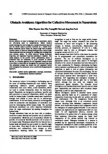
Measuring Data
Local Grid Map
Robot Pose T2
Goal Pose Sensing Range Behavior Selector
T1 (a) Detecting the obstacle using laser scanner Goal Tracking
E5
E1
E4
E2 Free Space Tracking
Sensing Range T2
Waiting
E3
Path Replanning
Contour Following
T1 Motion Commands (v, w)
(b) The obstacle is out of detection Fig. 1. The situation that the obstacle is out of detection during the avoidance procedure
Fig. 2. The reactive navigation structure
mounted on the robot has a limited sensing range from 0 to 180 degrees. This limited sensing range makes a situation that the obstacle is out of detection during the avoidance procedure (Fig. 1). To solve this problem, we make a local grid map around the robot and check the existence of the obstacles from 0 to 359 degrees. Then, the reactive navigation module computes the robot’s linear and rotate velocity for an obstacle avoidance using the information of the environment including measuring data, the robot pose, the goal pose and the local grid map (Fig. 2). The reactive navigation module has five different behaviors (GTM, FSTM, CFM, PRM, and WM). To compute the robot’s linear and rotate velocity for obstacle avoidance, the robot selects a proper behavior depending on the environment. A. Making Local Grid Map In this paper, we make the local grid map around the robot. The local grid map contains the accurate information of the surroundings and it is updated by laser scan data at 50ms
intervals. From this local grid map, we can check the existence of an obstacle from 0 to 359 degrees. To make the local grid map is divided into two steps: update (Table 1) and renew step (Table 2). In update step, we update the local grid map of the robot for the rear region that is not detected by the laser scanner mounted on the front of the robot. Using the method in table 1, we update the local grid map Gt-1 to Gt. Where Gt-1 and Gt are the occupancy grid map, μt −1 and μt are the robot poses at time t-1 and t. In renew step, we make the local grid map for the front region of the robot. The method that we use for renewing the local grid map is in Table 2. Fig. 3. shows the simulation result of making the local grid map. Fig. 3(a). is the measured laser scan data, and Fig. 3(b). is the local grid map after update and re-new steps. B. Reactive Navigation As the diagram in Fig. 2, the reactive navigation has five states and each state has an associated action that computes a
Table 1. the Update Step for Local Grid Map Table 2 the Renew Step for Local Grid Map
1. Update Local Grid Map (G t −1 , μt , μt −1 ) 2. G t ← empty set
1. Renew Local Grid Map (G t , μ t , S t )
3. for all occupied point Plocal ,t −1 in G t −1 do 4.
Transform Plocal | μ t −1 to Pg on the global coordinate
5.
Transform Pg to Plocal | μ t
2. for all masured points Pmeasure|μ t in S t do 3.
Transform Pmeasure|μt to Plocal |μt
4. endfor
6. endfor 7. G t ← {Plocal | μ t } ∪ G t
5. G t ← {Plocal |μt } ∪ G t
8. return G t
6. return G t
2063
C2
C1
C3 (a) G1 Pcol C2
G1 Fig. 3. Generating the local grid map and the distance histogram(Left : measured laser scan data, Right : generated local grid map)
G2
(1)
To select proper path from these gaps, we define a cost function. The cost function is show in Eq. (2).
f cost (θ i ,θ t −1 ) = k1 θ g − θ i + k 2 θ i − 90 + k 3 θ i − θ t −1
Pcounter C1
G3
motion command (v, w) to adapt the behavior to the navigational situation. v is the linear velocity of the robot and this is calculated depending on the distance to the obstacle in the front region; this is called “front distance” in this paper. Thus, robot velocity automatically decreases when an obstacle is close to the robot. w is the rotate velocity of the robot and this is calculated depending on the direction of the goal. Each module in reactive navigation calculates proper goal for computing w. To avoid obstacles, the behavior selector selects the most proper module depending on the environment and operates robot using v and w from the selected state. a) Goal Tracking Module: The Goal Tracking Module (GTM) controls the robot when no obstacle is on the robot’s path. So, GTM makes the robot track the optimal path from the path planning module. b) Free Space Tracking Module: If a front obstacle is closer than 2 m from the robot, then the reactive navigation module changes its state to Free Space Tracking Module (FSTM). FSTM is a kind of local path planner. To compute the obstacle free path, FSTM clusters the points in the local grid map based on the distance. Then, FSTM checks unoccupied regions between clusters; we called it a “gap.” If the gap size is larger than robot, we add that to the collision free candidates set. After making the collision free candidates set, FSTM checks whether the robot is able to move to each collision free candidate. Finally, FSTM decides which path is proper to avoid obstacle. The process to find the proper path is shown in Fig. 4. When the obstacle is in front of the robot (Fig. 4a), the local grid map is generated (Fig. 4b). The points on the local grid map are clustered based on the distance, then we can get the three clusters, C1, C2, and C3, after clustering (Fig. 4c). Then we find gaps, G1, G2, and G3, from clustering result (Fig. 4d), where Gi means the robot centered position of the ith gap between ith cluster and (i+1)th cluster.
Gi = ( xi , yi , θ i )
(c)
(b)
(2)
(d)
(f)
(e)
Fig. 4. Computing the collision free path where, θi is the direction of the ith gap in the robot centered
Ci Cj Pj
Pc
Pi
Fig. 5. Adjusting the avoid path using CFM coordinate, θ g is the direction of the robot’s goal, and θ t −1 is the direction of the selected path at time step t-1. Using this cost function, we select the proper path direction.
θ t = arg min f cost (θ i , θ t −1 )
(3)
i
In case of the environment in Fig. 4, the gap G1 is selected for the obstacle avoidance. If the robot approaches to G1 directly along the dotted line in Fig. 4e, it may be collide with cluster C2. To make collision free path, we modify the dotted line to the solid line in Fig. 4e. First, we find the point Pcol and Pcount. Pcol is the closest point to the direct path from the robot to the G1, and Pcount is the point on the line which is orthogonal to the dotted line passing the point Pcol. Then, we compute the center point between Pcol and Pcount, and modify the robot’s path and repeat it until the every distance from the point on the local grid map to the robot is larger than robot’s size (Fig. 4f). c) Contour Following Module: When the robot moves in a narrow corridor, the robot sometimes grazes along the obstacle, because the computed collision free path from FSTM is not the centerline of the corridor.
2064
The Contour Following Module (CFM) makes the robot navigate along the centerline of the corridor. When the robot follows the avoidance path (dotted line in Fig. 5) from the FSTM, if the obstacle approaches to the robot within predefined threshold, CFM checks the approaching obstacle from the lateral part of the robot. In Fig. 5, as the robot approaches to the cluster Cj, CFM computes the minimal distance to the Ci and Cj, and finds the closest point Pi, Pj in the each cluster. Then, CFM computes the center point between Pi and Pj. Finally, the robot traces the point Pc, and follows the path without any collision. d) Path Replanning Module: The Path Replanning Module (PRM) computes a detour path and orders the mobile robot to take a detour. If no gap between clusters exists in front of the robot on the local grid map, the robot regards every obstacle in front of it as walls and registers them in the map. Then, the robot recomputes the path to the target position. e) Wait Module: When no detour path exists, the WM makes robot wait until the obstacle moves.
A
B C
Fig. 6. Pioneer DX2 mobile robot used in the experiments, where, A is a Bumblebee stereo camera, B is a Pentium IV 1.86GHz computer, and C is a HOKUYO URG-04LX laser range finder
III. EXPERIMENTAL RESULTS The proposed method was implemented on our mobile robot (Fig. 6). The robot used in experiment is an ActiveMedia Pioneer DX2 mobile robot equipped with a HOKUYO URG04LX laser range finder and a BUMBLEBEE stereo camera. For sensing the environment, the robot used the laser range finder, which detect the distance to the obstacle around robot and its sensing range is from 0°to 180°. The experiment was carried out in several simulated and real environments including a narrow and complex environment, a dead-end trap, and high dynamic situation and the robot was able to navigate in a corridor without any collision with obstacles (Fig. 7). In the narrow path environment (Fig. 7a), the robot follows the center of the path. In the U-shaped trap environment (Fig. 7b), the robot detected the trap and avoided it successfully. Even in the crowded environment (Fig. 7c), the robot also avoided the obstacles without any collision. In contrast to earlier experiments, several avoidance paths existed in the crowded environment, however the robot arrived at the goal through the shortest path. The minimum distance between obstacles in the crowded environment is about 0.6 m and the robot which has 0.5m diameter, could pass that avoidance path and the minimum path width that the robot could pass is about 0.6m and it is 0.1m larger than the robot’s diameter. The robot could also react to the obstacles in real time, because the processing time for computing the collision free path is 0.015 ms. IV. DISCUSSION We discuss next the advantages of this method compared existing techniques on the basis of the difficulties shown in the experimental results. The local trap situations due to U-shape obstacles are overcome with this method. Our robot does not move to the local trap because FSTM places subgoals outside of these
obstacles (Fig 7b). Thus our robot can avoid obstacles mostly because it does not fall into trap. In addition to this our robot selects motion directions far away from the goal direction when required. This is because the subgoals can be placed in any location in the search space. In other words, any deviation from the goal direction can be obtained with this method. For example, when the robot met the local trap, the only way to reach the target was to move to the right, which implies a direction far from the goal direction. In the narrow path environment, the passage is very narrow. However, the robot follows the center of the path because the CFM places the subgoals at the center of the path (Fig 7a). This issue was critical when moving in narrow corridors, because many obstacles : a cabinet, a dustbin, a desk and a chair, are placed on the edge of the corridor and this makes the corridor narrower. In the crowded environment, the robot moves to the goal with the shortest path (Fig. 7c), because the smallest width of passage our robot can go through is 0.6 m; this is almost the same as the robot’s radius (= 0.5m). The robot could also react to the obstacles in real time, because the processing time for computing the collision free path is 0.015 ms. The mobile robot navigation system described in this paper can be working for obstacle avoidance in environments consisting of dynamic as well as static obstacles, because our method can compute the avoid path in real time. Also our method can make the robot navigate in very dense, clutterd, and complex scenarios which are a challenge for many other methods. Although our method works for only circular and holonomic robots, scope for future research includes extending our method for other shapes robot with different kinematic and dynamic constraints.
2065
U-shaped obstacle
(a)
(b)
(c) Fig. 7. Experimental Results for the reactive navigation. (a) The trajectory of the narrow environment (b) The trajectory of the U-shaped trap environment (c) The trajectory of the crowded environment. [6]
ACKNOWLEDGMENT This work was supported by grant No. RTI04-02-06 from the Regional Technology Innovation Program of the Korean Ministry of Commerce, Industry and Energy (MOICE). REFERENCES [1]
[2]
[3]
[4]
[5]
[7]
[8]
[9]
S. Thrun, M. Bennewitz, W.Burgard, A.B. Cremers, F. Dellaert, and D. Fox, “MINERVA: A Second-Generation Museum Tour-Guide Robot,” Proc. of IEEE Int. Conf. Robotics and Automation(ICRA ’99), pp19992005, 1999. R.Simmons, J. Fernandez, R. Goodwin, S. Koenig, and J. O’Sullival, “Xavier: An Autonomous Mobile Robot on the Web,” IEEE Robotics and Automation Magazine, Vol. 7, No. 1, pp. 33-39, 2000. R. Siegwart, K. O. Arras, S. Bouabdallah, D. Burnier, G. Froidevaus, X. Greppin, B. Jensen, A. Lorotte, L. Mayor, M. Meisser, R. Phillippsen, R. Piguet, G. Ramel, G. Terrien, and N. Tomatis, “Robox at Expo.02: A large-scale installation of personal robots,” Robot. Auton. Syst., Vol.42, pp. 203-222, 2003 J. Borenstein, “Real-Time Obstacle Avoidance for Fast Mobile Robots,” IEEE Trans. Systems, Man and Cybernetics, Vol. 19, No. 5, pp. 11791187, 1989. J. Borenstein and Y. Koren, “The Vector Field Histogram: Fast Obstacle Avoidance for Mobile Robots,” IEEE Journal of Robotics and Automation, Vol. 7, No. 3, pp. 278-288, 1991.
[10]
[11]
[12]
[13]
2066
R. Philippsen, and R.Siegwart, “Smooth and Efficient Obstacle Avoidance for a Tour Guide Robot,” Proc. of IEEE Int. Conf. Robotics and Automation(ICRA ’03), pp. 446-451, 2003. N.Y. Ko and R. Simmons, “The lane-curvature method for local obstacle avoidance,” Proc. of IEEE Int. Conf. Intelligent Robots and Systems (IROS ’98), 1998. D.Fox, W.Burgard, and S. Thrun, “the dynamic window approach to collision avoidance,” IEEE Robotics and Automation Magazine, Vol. 4, No. 1, pp23-33, 1997. J.C.Latombe, and J.Barraquand, “Robot Motion Planning: A Distributed Presentation Approach,” Int. Journal of Robotics Research, vol. 10, pp.628-649, 1991. M. Khatib, H. Jaouni, R. Chatila, and JP. Laumond, “Dynamic path modification for car-like nonholonomic mobile robots,” Proc. of IEEE Int. Conf. Robotics and Automation(ICRA ‘97), pp. 2920-2925, 1997. M. Drumheller, “Mobile robot localization using sonar,” IEEE Trans. on Pattern Analysis and Machine intelligence, Vol. PAMI–9, pp. 323–332, 1987. M.Betke and L.Gurvits, “Mobile Robot Localization Using Landmarks,” IEEE. Trans. Robotics and Automation, Vol. 13, No. 2, pp 251-263, 1997. S.Thrun, D.Burgard, and D.Fox, Probabilistic ROBITICS, The MIT Press, Cambridge, 2005.