Vesna Gardaševic, Ralf R. Müller, Daniel J. Ryan, Lars Lundheim and Geir E. ... Email: {vesna.gardasevic, mueller, daniel.ryan, lundheim, oien }@iet.ntnu.no.
ISITA2010, Taichung, Taiwan, October 17-20, 2010
Lattice-Reduction Aided HNN for Vector Precoding Vesna Gardasevi´c, Ralf R. M¨uller, Daniel J. Ryan, Lars Lundheim and Geir E. Øien Department of Electronics and Telecommunications The Norwegian University of Science and Technology 7491 Trondheim, Norway Email: {vesna.gardasevic, mueller, daniel.ryan, lundheim, oien }@iet.ntnu.no Abstract—In this paper we propose a modication of the Hopeld neural networks for vector precoding, based on Lenstra, Lenstra, and Lov`asz lattice basis reduction. This precoding algorithm controls the energy penalty for system loads α = K/N close to 1, with N and K denoting the number of transmit and receive antennas, respectively. Simulation results for the average transmit energy as a function of α show that our algorithm improves performance within the range 0.9 ≤ α ≤ 1, between 0.4 dB and 2.6 dB in comparison to standard HNN precoding. The proposed algorithm performs close to the sphere encoder (SE) while requiring much lower complexity, and thus, can be applied as an efcient suboptimal precoding method.
I. I NTRODUCTION We consider the application of precoding algorithms in a broadcast MIMO system, typically consisting of a transmitter with N antennas and K receivers. The aim of these methods is to improve the system performance, and to provide simplied receiver design. Precoding algorithms can be based on linear or a combination of linear and nonlinear transformations. The main advantage of linear precoding (e.g., [1], [2]) is in its low-complexity implementation. However, this method does not provide good performance unless the load is very small. In order to obtain practical precoding algorithms providing higher data rates, methods that combine linear and nonlinear algorithms have been proposed (e.g., [3]). One approach in nonlinear precoding is to apply Tomlinson-Harashima precoding (THP) based on the zero forcing (ZF THP) [3] or the minimum mean square error (MMSE) (MMSE THP) (e.g., [4]) criterion. Further performance improvement is achieved by vector perturbation [5], a popular precoding method that is a generalization of the THP concept. In vector perturbation, the transmit signal is composed of a sum of the data symbols and a complex perturbation vector. The perturbation vector is chosen such that the transmit power is minimized. Numerical results show that vector perturbation achieves signicant performance enhancement for all signal-to-noise ratio (SNR) regions. However, state-of-the-art vector perturbation employs a sphere encoder (SE) [6] with exponential expected complexity [7] for the search of the perturbation vector. Reductions in the computational complexity of vector precoding have been provided by algorithms based on lattice-basis reduction (LR) (e.g., [8], [9]). Precoding based on LR algorithms that employ the polynomial-time Lenstra, Lenstra, and Lov`asz (LLL) algorithm [10] have been investigated in e.g., [9]. The LLL algorithm calculates an alternative basis with less correlated, short vectors, such that detection and precoding are
improved due to less power enhancement. Another practical algorithm is convex relaxation (CR) precoding proposed in [11]. CR precoding is an algorithm of polynomial complexity, where the minimization of the transmit power is formulated as a convex optimization problem. In this paper we extend our results on HNN precoding [12] by implementing a LLL-LR-based modication of the HNN precoding algorithm. Sole HNN precoding as investigated in [12] provides performance close to the SE precoding within the load 0 < α ≤ 0.6, where the load α = K/N is the ratio of the number of receive antennas K to the number of transmit antennas N . It has been shown that sole HNN exhibits a degradation for loads close to 1. We show that the LLL-LR HNN obtains improvements compared to the performances of sole HNN precoding within the system load 0.9 ≤ α ≤ 1. LLL-LR improves performance for HNNs, while for the SE it only moderates complexity, still keeping it exponential. For example, for K = 4, the LLL-LR HNN achieves performance very close to the performance of the SE, while keeping essentially the same complexity as linear precoding. We investigate the performances of LLL-LR HNN by simulations. Numerical results for the LLL-LR HNN will be given in terms of the average transmit power as a function of the system load α, for a MIMO system with K = 4, K = 8, and K = 16 receive antennas. We compare numerical results with the performances of: the sole HNN for vector precoding for the same number of receive antennas, the convex relaxation (CR) [11] for K → ∞, the SE where K → ∞ [13], and with numerical results for the SE lattice precoding, where each information bit is represented by L = 2 redundant symbols. Notation: Matrices and vectors are denoted by uppercase boldface and lowercase boldface letters, respectively and scalars by ordinary letters. (·)−1 , (·)T , (·)+ , and (·)† denote the inverse, the transpose operator, the pseudo-inverse and the conjugate transpose, respectively. The Euclidean norm is denoted by � · �, inner product of two vectors by �·�, rounding to the nearest integer value by �·�, and absolute value by | · |. � and � prex denote the real and imaginary parts of a complex matrix and vector. II. SYSTEM MODEL We consider a Gaussian broadcast MIMO channel with a single transmitter with N antennas, and K non-cooperative receivers. Each receiver is equipped with a single antenna. In
c 2010 IEEE 978–1–4244–6017–5/10/$26.00 � 37
our scenario the number of transmit antennas is greater than or equal to the number of receive antennas, K ≤ N . Perfect channel state information (CSI) is available at the transmitter. The MIMO system is modeled as ˜˜ r˜ = H t+n ˜
This optimization problem belongs to the class of nonconvex optimization problems in a high dimensional lattice, and it is known to be NP-hard. In order to provide a lower complexity suboptimal solution for the optimization problem (5), in the next section, we proceed with the derivation of the LLL-LR HNN precoding algorithm for the selection of the optimal vector x.
(1)
where the transmit vector is denoted by ˜ t = [t˜1 , ˜t2 , · · · , t˜N ]T , the receive vector is denoted by r˜ = [˜ r1 , r˜2 , · · · , r˜K ]T , and elements of the white Gaussian noise vector n ˜ = [˜ n1 , n ˜ 2, · · · , n ˜ K ]T are complex-valued Gaussian random variables with zero-mean and unit variance. The vector s˜ = [˜ s1 , s˜2 , · · · , s˜K ]T contains quaternary phase-shift keying (QPSK) data symbols, where the s˜i entries are from the set ˜ = {1 + j, −1 + j, 1 − j, −1 − j}, for i = 1, 2 . . . , K. The S ˜ are independent elements of the K × N channel matrix H and identically distributed (i.i.d.) complex-valued Gaussian random variables with zero-mean and unit variance. The complex-valued model of the system (1) can be represented as a corresponding 2K real-valued system. The real and imaginary parts of the complex-valued matrix and vectors are included into the system model; thus the 2K ×2N real-valued MIMO system (1) is reformulated as �
�˜ r �˜ r
�
=
�
˜ �H ˜ �H
˜ −�H ˜ �H
��
�t˜ �t˜
�
+
�
�˜ n �˜ n
A. Lattice Basis Reduction Algorithm The search for a less correlated basis with short vectors in a lattice set can be carried out by lattice reduction algorithms [14], for example the Minkowski or LLL reduction algorithms. In order to proceed with the implementation of the precoding algorithm based on lattice basis reduction, denitions [14] and a brief introduction on general lattices will be given in this subsection. �d A lattice or Z-module, denoted by L = i=1 Zbi = �d { i=1 λi bi : λ1 , · · · , λd ∈ Z} is a set of all integer combinations of the vectors b1 , b2 , · · · , bd ∈ Rn , where n ≥ d, and d is the lattice dimension. If the vectors (b1 , b2 , · · · , bd ) are linearly independent, they constitute a basis of the lattice. Innitely many different basis can be constructed for d ≥ 2. Let B be the matrix B = [b1 , b2 , · · · , bd ], consisting of the column vectors b1 , b2 , · · · , bd . The lattice basis obtained by the LLL algorithm is not necessarily the best one, but it is only by a certain factor worse than the best basis. Applying the LLL algorithm to the columns of B, a new reduced basis L(B), with basis vectors ˇ b1 , ˇ b2 , · · · , ˇ bd is obtained. Those two lattice bases are related to each other via an unimodular transformation, that is B red = BU , where U is a unimodular matrix, i.e. a matrix consisting of integers, with normalized determinant | det(U )| = 1. Let the LR of the pseudo-inverse H + be denoted by + H+ red = H U , where U is a unimodular matrix. Since + the basis H red has better properties in terms of basis vector length and orthogonality, less average transmitted energy will be required. We will at the moment neglect the noise in (1) and consider the received vector given by HH + U x. Given that the data vector is represented by the shifted lattice 2Z + 1, the 2K-dimensional received vector r should be represented by a shifted lattice as well, in order to provide interference-free transmission. Let 1 be the 2K vector consisting of ones. For any vector x ∈ (2Z + 1)2K , we have U x ∈ (2Z)2K + U 1. Thus, an unimodular matrix acting on a shifted lattice does not distort the lattice, but only shifts it. Assuming this constant shift U 1 to be known to the receiver, it can easily be compensated for.
�
The real equivalent of the data symbol vector s˜, denoted by s, is mapped to the vector x= [x1 , x2 , · · · , x2K ]T , obtained as a solution of a transmit energy minimization to be performed. The entries of the real equivalent data vector s = [s1 , s2 , · · · , s2K ]T are binary phase-shift keying (BPSK) modulated symbols that belong to the set S = {±1}. For each BPSK symbol, we allow for a redundant representation consisting of two symbols, such that the relaxed alphabet sets are given by: B1 = {1, −3} and B−1 = {−1, 3}. In the linear precoding step, the transmit vector t is premultiplied with the pseudo-inverse of the channel matrix H, denoted by the matrix T , i.e. t = Tx
(2)
T = H + = H † (HH † )−1
(3)
where T is given as
and the 2K real-valued vector x has been obtained as a solution of the optimization problem for the transmit energy minimization. We start by formulating the expression for the minimization of the transmit energy for the system (1), and next we consider the optimization problem of the transmit energy minimization. The optimal vector x is obtained as a solution to the optimization problem: x∗ =
argmin x∈Bs1 ×···×Bs2K
�T x�2 =
argmin x∈Bs1 ×···×Bs2K
III. HOPFIELD NEURAL NETWORKS The HNN [15] is modeled as a system consisting of interconnected signal processing units − neurons, an external threshold value θi , and an activation function. Each connection between two neurons is determined by a weight, and the set of all weights in the HNN is represented by a weight matrix W . The choice of the weight matrix W depends on the underlying system that is modeled by the HNN. An input signal at a
x† (HH † )−1 x (4) 38
neuron is usually a binary valued signal {1, −1} or {1, 0}. A task of an external threshold value θi is to control an amplitude of the signal at the input of the activation function. In the HNN, the amplitude of the sum of a linear combination of the weighted input states and the threshold θi is limited by an activation function. The HNN employs feedback, and the output of the activation function is sent at the input of the neurons.The activation function can be implemented by various functions, for example: hard limiter (threshold) transfer function, hyperbolic tangent (tanh), sigmoid and other functions. The mathematical model of discrete HNN [15] is given in the form �K � � (l+1) (l) vj =f wji vi + θj (5)
The LLL-LR HNN precoding algorithm works as follows: The LLL algorithm is applied to the pseudo-inverse H + of the + channel matrix, and H + red = H U is obtained. The transmit + vector is given by t = H red x, and the optimization problem + † + 2 † is formulated as minimizing �H + red x� = x (H red ) H red x over the constraint set x ∈ Bs1 × · · · × Bs2K . The LLL algorithm is shown in Table I. TABLE I LLL A LGORITHM .
Algorithm 1: LLL Algorithm Input: Lattice basis (b1 , b2 , · · · , bd ) 1: Gram-Schmidt orthogonalization step 2: Compute the Gram-Schmidt orthogonal basis: 3: ˇ b1 , ˇ b2 , · · · , ˇ bd
i=1
where l = 1, 2 · · · , denotes the number of iterations run by the HNN, i = 1, 2 . . . , K, j = 1, 2 . . . , K, the network states are denoted by vj , wji are the assigned weights between neurons j and i, f(·) is an activation function, and θj is a threshold value. The energy function of the HNN is described by K
E=
K
7: 8: 9:
K
� 1 �� wij vi vj + vi θi 2 i=1 j=1
4: Size Reduction step 5: for 2 ≤ i ≤ d do 6: for i − 1 ≤ j ≤ 1 do
(6)
10: 11: 12:
i=1
The application of the HNN in optimization problems is based on the fact that the energy function (6) monotonically decreases or remains the same with the change of the states, resulting in the local minima of the energy function. The computational complexity of the pure HNN is given by O(K 2 ), where for every symbol vector we need to calculate a matrixvector product per iteration. In vector precoding based on the HNN [12], the HNN is applied for searching for the optimal vector x in (5) that minimizes the transmit energy (6). There is a clear correspondence between (3) and (5), where vector x in (3) corresponds to the output vector v of the HNN in (5), and −1 the matrix (HH † ) (except for its diagonal) corresponds to the weight matrix W (5) with entries wij . We consider in our work the application of the polynomialtime LLL algorithm [10]. The LLL algorithm and its modications (e.g., [16]) that obtain performance improvements, have been successfully used in various applications, when the approximation of the shortest vector problem or closest vector search is required, e.g., number theory, computer algebra, cryptography, signal detection and precoding (e.g., [9]) problems, etc. The LLL algorithm consists of vector length reduction, and vector re-ordering steps, performed until no further enhancement in vector size reduction is obtained. The basis is said to be an LLL-reduced basis if the conditions |µi,j | ≤ 0.5, where i = 1, 2 . . . , d, j ≤ i, and δ�ˇ bi �2 ≤ �µi+1,iˇ bi + ˇ bi+1 �2 , where µi,j = ��bi , ˇ bj ��/�ˇ b j �2 , δ ∈ (0.25, 1) and i = 1, 2 . . . , d are fulllled. Smaller values of δ yield faster convergence, while larger values of δ provide reduced basis with better properties in terms of orthogonality and lengths of basis vectors.
Dene: µi,j = ��bi , ˇ bj ��/�ˇ bj �2 bi ← bi − �µi,j �bj Swap the vectors: if �ˇ bi−1 �2 > 2�ˇ b i �2
then Swap the vectors bi−1 and bi ˇ bi ↔ ˇ bi−1
13: 14: i ← i−1 15: else 16: i ← i+1 17: end 18: Go to Gram-Schmidt orthogonalization step 19: end 20: end 21: Output: LLL-reduced basis ˇ b1 , ˇ b2 , · · · , ˇ bd
The algorithm of the HNN based on the lattice basis reduction for vector precoding is shown in Table II. The activation function tanh is applied on the weighted combination of the input signal s, where the weights are + † entries of the matrix (H + red ) H red . The activation function (l) generates a soft decision vi , where l = 1 is the starting iteration, and the maximum number of iterations is Imax . In each iteration the current soft value is subtracted from the soft value from the previous iteration, until the number of iterations exceeds the maximum number of iterations Imax . IV. NUMERICAL RESULTS In this section, we illustrate the behavior of the proposed algorithm in terms of the transmit energy as a function of the ratio α = K/N . Simulation results are compared with the performances of: analytical results for the SE (the number of the redundant representations of each information bit is L = 2), when K → ∞ [13], simulation results for the SE 39
TABLE II H OPFIELD N EURAL N ETWORK FOR V ECTOR P RECODING .
12
Algorithm 2: Hopeld Neural Network for Vector Precoding
11
1: Input: Set H , v = s, l = 1, Imax
10
2: 3:
Set H + = H † (H H † )−1 Generate LLL (H + )
9
4:
H+ red
E [dB]
+
= LLL (H )U
5: Set W = (H H † )−1 6: HNN algorithm 7: Dene: fsj (y) = −sj + 2 tanh (2 (y + sj )) 8: while l ≤ Imax do 9: for 1 ≤ j ≤ 2K do 10: Calculate � � 2K wji (l) (l) 11: vj = fsj (− j−1 i=1 wjj vi − i=j+1 12: end 13: end 14: for 1 ≤ j ≤ 2K do 15: xj = −sj + 2 · sign(vj + sj ) 16: end 17: Output: x
8
HNN: K=4 HNN: K=8 HNN: K=16 LLLíLR HNN: K=4 LLLíLR HNN: K=8 LLLíLR HNN: K=16 CR: K → ∞ SE (L=2): K → ∞
7 6 5 wji wjj
(l−1) vi )
4 0.5
Fig. 1.
11 10 9 E [dB]
0.7
0.8
α =K/N
0.9
1
HNN Algorithm. The average transmit energy as a function of α.
12
(L = 2), analytical results for CR [11] when K → ∞, and the sole HNN algorithm for vector precoding [12]. The channel matrix H has been modeled with i.i.d. zeromean Gaussian entries with unit variance. The number of different channel realizations for the system sizes K = 4 and K = 8 was 10 000, while for K = 16 there were 5 000 different channels. For each realization of the channel matrix H, the number of the HNN iterations was set to be Imax = 40. The number of receive antennas was chosen to be: K = 4, K = 8, and K = 16. Fig. 1 shows the performances of the sole HNN and the LLL-LR HNN precoding algorithms. In Fig. 2 the performances of the LLL-LR HNN precoding algorithm and the SE are compared, for the same simulation setting. The sole HNN and the LLL-LR HNN algorithms in Fig. 1 provide similar performances for loads in the range 0.5 < α ≤ 0.7. A gradual increase in the performance degradation of the sole HNN algorithm was observed in the range of 0.7 ≤ α ≤ 0.9. Within this range the LLL-LR provides performance enhancement, and for α = 0.9 the LLL-LR HNN outperforms the sole HNN by 1 dB, 0.9 dB, and 0.4 dB, for K = 4, K = 8, and K = 16, respectively. For loads close to 1, the performance of the sole HNN degrades in comparison to the SE. This is due to the fact that the lattice precoding exhibits replica symmetry breaking (RSB) [13] in a system where the number of transmit and receive antennas is close to each other, while the HNN does not model well the RSB problems. We observe that within the range 0.9 ≤ α ≤ 1, where the sole HNN suffered from severe performance degradation, the LLL-LR HNN controls the energy penalty exhibited by the HNN. Fig. 2 indicates the performances of the LLL-LR HNN
0.6
8
LLLíLR HNN: K=4 LLLíLR HNN: K=8 LLLíLR HNN: K=16 SE (L=2): K=4 SE (L=2): K=8 SE (L=2): K=16 CR: K → ∞ SE (L=2): K → ∞
7 6 5 4 0.5
0.6
0.7 0.8 α =K/N
0.9
1
Fig. 2. LLL-LR HNN Algorithm. The average transmit energy as a function of α.
algorithm in comparison to the SE. For example, for α = 0.9 and K = 4, the SE outperformes the LLL-LR HNN by only 0.2 dB, as indistiguishably well as SE while being only of cubic complexity. V. COMPUTATIONAL COMPLEXITY In this subsection we compare the computational complexity of the proposed algorithm, and algorithms used for comparison. The algorithms considered in this work require a matrix inversion to calculate the pseudo-inverse. The calculation of the matrix inverse is of O(K 3 ) complexity. All the additional complexity introduced in the system, that has complexity less 40
than cubic, will be negligible in comparison to the matrix inversion. The LLL algorithm obviously has complexity O(K 2 ) per iteration. Recent results [17] on the worst and average case complexity of the LLL provided new insights on the complexity of the LLL applied to a wireless MIMO system. It has been shown that the number of the LLL iterations is not upper-bounded, when the lattice reduction is carried out on an i.i.d. Rayleigh channel matrix. The average complexity of the LLL in an i.i.d. Rayleigh channel, in terms of the average number of the LLL iterations, is polynomial with respect to the lattice dimension. Research on the convergence time of neural networks (e.g., [18], [19], [20] ) has closely followed the active research eld on various models and diverse attractive applications of neural networks. There are various realizations of HNN, for example: continuous or discrete time, feedforward or recurrent model, with discrete or analog activation function, nite or innite network size, asynchronous or synchronous network. The HNN computational complexity has been analyzed depending on the network model and its applications. Some of the results on the computational complexity have been generalized. First we consider the results on the convergence of a symmetric HNN applied for an energy minimization that we used in the proposed algorithm, in terms of convergence time. In the worst case the HNN convergence time may be exponential, but that under some mild conditions, the binary HNN converges in only O(log log K) parallel steps in the average case. For the binary HNN with polynomial weight size, convergence time is polynomial with absolute error less �K � K then 0.243 i=1 j=1 |wij |. The expected complexity of the SE [7], with respect to the number of jointly detected symbols is exponential. However, the complexity of SE although high, for the applications of the moderate size can be considered as a practical algorithm. CR is based on the application of the convex optimization solvers of polynomial complexity. The CR precoding is carried out by a quadratic solver, that has the computational complexity of O(K 3.2 ).
R EFERENCES [1] R. F. Fischer, Precoding and Signal Shaping for Digital Transmission . New York , NY , USA: John Wiley & Sons, Inc., 2002. [2] C. Peel, B. Hochwald, and A. Swindlehurst, “A Vector-Perturbation Technique for Near-Capacity Multiantenna Multiuser Communicationpart I: Channel Inversion and Regularization,” Communications, IEEE Transactions on, vol. 53, no. 1, pp. 195–202, Jan. 2005. [3] C. Windpassinger, R. Fischer, T. Vencel, and J. Huber, “Precoding in Multiantenna and Multiuser Communications,” Wireless Communications, IEEE Transactions on, vol. 3, no. 4, pp. 1305–1316, July 2004. [4] M. Joham, J. Brehmer, A. Voulgarelis, and W. Utschick, “Multiuser spatio-temporal tomlinson-harashima precoding for frequency selective vector channels,” in Smart Antennas, 2004. ITG Workshop on , March 2004, pp. 208–215. [5] B. Hochwald, C. Peel, and A. Swindlehurst, “A Vector-Perturbation Technique for Near-Capacity Multiantenna Multiuser CommunicationPart II: Perturbation,” IEEE Trans. Commun., vol. 53, no. 3, pp. 537–544, March 2005. [6] U. Fincke and M. Pohst, “Improved methods for calculating vectors of short length in a lattice, including a complexity analysis,” Mathematics of Computation, vol. 44, no. 170, pp. 463–471, 1985. [7] J. Jalden and B. Ottersten, “On the Complexity of Sphere Decoding in Digital Communications,” IEEE Trans. Signal Processing, vol. 53, no. 4, pp. 1474–1484, April 2005. [8] M. Taherzadeh, A. Mobasher, and A. K. Khandani, “Communication Over MIMO Broadcast Channels Using Lattice-Basis Reduction,” IEEE Trans. Inf. Theory, vol. 53, no. 12, pp. 4567–4582, 2007. [9] C. Windpassinger, R. Fischer, and J. Huber, “Lattice-reduction-aided broadcast precoding,” Communications, IEEE Transactions on, vol. 52, no. 12, pp. 2057–2060, Dec. 2004. [10] A. K. Lenstra, H. W. Lenstra, Jr., and L. Lov´asz, “Factoring Polynomials with Rational Coefcients,” Math. Ann., vol. 261, no. 4, pp. 515–534, 1982. [11] R. R. M¨uller, D. Guo, and A. L. Moustakas, “Vector Precoding in High Dimensions: A Replica Analysis,” IEEE J. Sel. Areas Commun., vol. 26, no. 3., p. 530540, Apr. 2008. [12] V. Gardasevi´c, R. R. M¨uller, and G. E. Øien, “Hopeld Neural Networks for Vector Precoding,” International Zurich Seminar on Communications (IZS), Zurich, Switzerland, March 2010. [13] B. M. Zaidel, R. R. M¨uller, R. de Miguel, and A. L. Moustakas, “On Spectral Efciency of Vector Precoding for Gaussian MIMO Broadcast Channels,” Proc. IEEE 10th Int. Symp. Spread Spectrum Techniques and Applications (ISSSTA), pp. 232–236, Aug. 2008. [14] J. V. Z. Gathen and J. Gerhard, Modern Computer Algebra. New York, NY, USA: Cambridge University Press, 2003. [15] A. Cochocki and R. Unbehauen, Neural Networks for Optimization and Signal Processing. New York, NY, USA: John Wiley & Sons, Inc., 1993. [16] P. Q. Nguyen and D. Stehl´e, “An LLL Algorithm with Quadratic Complexity,” SIAM J.. of Computing, vol. 39, no. 3, pp. 874–903, 2009. [17] J. Jald´en, D. Seethaler, and G. Matz, “Worst- and Average-Case Complexity of LLL Lattice Reduction in MIMO Wireless Systems,” in IEEE International Conference on Acoustics, Speech and Signal Processing (ICASSP), Las Vegas, USA, March 2008, pp. 2685–2688. ma, “Energy-based Computation with Symmetric Hopeld Nets,” in [18] J. S´ Limitations and Future Trends in Neural Computation, NATO Science Series: Computer and Systems Sciences, vol. 186. IOS Press, 2003, pp. 45–69. ma, P. Orponen, and T. Antti-Poika, “On the Computational [19] J. S´ Complexity of Binary and Analog Symmetric Hopeld Nets,” Neural Comput., vol. 12, no. 12, pp. 2965–2989, 2000. [20] G. Serpen, “Hopeld Network as Static Optimizer: Learning the Weights and Eliminating the Guesswork,” Neural Processing Letters, vol. 27, no. 1, pp. 1–15, 2008.
VI. CONCLUSIONS We have proposed a modication of the HNN for vector precoding, based on LLL, in order to enhance the performance of the HNN precoding algorithm, particulary for loads 0.9 ≤ α ≤ 1. The simulation results indicate that the LLL-LR HNN outperforms the sole HNN precoding algorithm for loads within this range, for the simulated number of receive antennas K. Generalizations to higher order modulations are trivial if Gray mapping is used. For the load within 0.9 ≤ α ≤ 1 the LLL-LR HNN achieves an enhancement in performance between 0.4 dB and 2.6 dB, improving the performances and controlling the energy penalty of the HNN precoding, that are degraded for loads 0.9 ≤ α ≤ 1. For K = 4 and unit load, LLL-LR HNN performs indistiguishably close to the SE, while being only of cubic complexity.
41