Learning and predicting time series by neural networks

Learning and predicting time series by neural networks Ansgar Freking and Wolfgang Kinzel

arXiv:cond-mat/0202537v1 [cond-mat.dis-nn] 28 Feb 2002

Institut f¨ ur Theoretische Physik und Astrophysik, Universit¨ at W¨ urzburg, Am Hubland, 97074 W¨ urzburg, Germany

Ido Kanter Minerva Center and Department of Physics, Bar-Ilan University, Ramat-Gan 52900, Israel Artificial neural networks which are trained on a time series are supposed to achieve two abilities: firstly to predict the series many time steps ahead and secondly to learn the rule which has produced the series. It is shown that prediction and learning are not necessarily related to each other. Chaotic sequences can be learned but not predicted while quasiperiodic sequences can be well predicted but not learned. PACS numbers: 05.20.-y,05.45.TP,87.18.Sn

Neural networks are able to learn a rule from a set of examples. This paradigm has been used to construct adaptive algorithms – named artificial neural networks – which are trained on a set of input/output patterns generated by an unknown function. After the training process, the network can reproduce the patterns, but is also has achieved generalization: it has obtained some knowledge about the unknown function. In the simplest case the unknown function is a neural network itself, the “teacher”. A different neural network with an identical architecture, the “student”, is trained on a set of examples produced by the teacher. This so called ”student/teacher” scenario has been intensively studied using models and methods of statistical physics [2, 3, 4]. Recently these methods have also been applied to learning and generation of time series [5, 6, 7, 8, 9]. The main result of these theoretical investigations is that as the student network receives more information it increases its similarity to the weights of the teacher network. When the number of training examples is much larger than the number of parameters of the teacher, the student is almost identical to the teacher and the generalization error is close to zero. In this article we show that this fundamental relation between learning and generalization is violated when a neural network is trained on a time series. We present a class of networks with almost perfect prediction of the series and almost zero information about the rule. The opposite case is found, as well: A network cannot predict a time series although it is almost identical to the rule generating the series. Hence the intuitive deduction that learning a rule leads to good generalization and good generalization indicates good knowledge about the rule is violated both ways when a neural network is trained on a time series. We find this phenomenon already for a simple perceptron, a neural network with a single layer of synaptic weights, given by the equation o = g (w · S). Here w = (w1 , w2 , ..., wN ) is the vector of synaptic weights, S = (st−1 , st−2 , ..., st−N ) is the input of the network (window of the time series), o is the output value and N is the size of the network. In the following we will study different transfer functions g(x). Such a perceptron can be used as a sequence generator (teacher with weights wT ) as well as a network being trained on a time series (student with weights wS )[5]. The sequence is generated by a teacher network with random weights, starting from random initial conditions (sN , sN −1 , ..., s1 ); hence it is defined by the equation   N X (1) st = g  wjT st−j  j=1

We define a time t0 in such a way that the sequence is stationary for any t > t0 . Here, ”stationary” means that the sequence lies on its attractor. The transient, which is of O(N ) is not included in the training examples. The training error is calculated from the absolute value of the deviation between the sequence st and the corresponding output ot of the student: t0 +T 1 X |st − ot | T →∞ T t=t +1

ǫ = lim

(2)

0

This is the average error of a one-step-prediction of the student on the time series. Perfect training leads to zero error ǫ, meaning that each number of the sequence is correctly reproduced: st = ot . The student’s knowledge about the unknown parameters is measured by the overlap R between the weight vectors

2 of the teacher and the student: R=

wT · wS |wT ||wS |

(3)

If the transfer function is continuous, it is also important that the two vectors coincide in their length QS = QT with Q = |w|. First we discuss the Boolean perceptron, g(x) = sign(x), of size N which has generated a periodic bit sequence [5, 7]. The teacher perceptron has random weights with zero bias, and the cycle is related to one component of the power spectrum of the weights. The student network is trained using the perceptron learning rule: ∆wiS =

1 N st

st−i

if st

N X

wjS st−j < 0;

j=1

∆wiS

= 0 else.

(4)

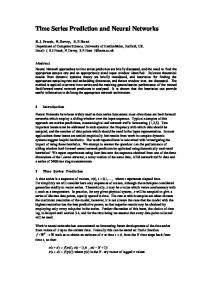
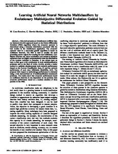
For this algorithm there exists a mathematical theorem [2]: If the set of examples can be generated by some perceptron then this algorithm stops, i.e. it finds one out of possibly many solutions. Since we consider examples from a bit sequence generated by a perceptron, this algorithm is guaranteed to learn the sequence perfectly. The network is trained on the cycle until the training error is zero. Hence the student network can predict the stationary sequence perfectly. It turns out that the overlap between student and teacher remains small, in fact it is zero for infinitely large networks, N → ∞. Although the network predicts the sequence perfectly, it does not gain much information on the parameters of the network which has generated this sequence. 0.3 0.25

R

0.2 0.15 0.1 0.05 0 0

0.05

0.1

0.15

0.2

0.25

0.3

N−1/2 FIG. 1: Final overlap R between student and teacher network after training, as a function of the size N of the network. The standard error-bars result from M = 100 individual runs. A linear fit of R vs. N −1/2 supports the statement that R → 0 for N → ∞.

This situation seems to be different in the case of a continuous perceptron. Inverting Eq. (1) for a monotonic transfer function g(x) gives N linear equations for N unknowns wiT . If all patterns are linearly independent then batch training, using N windows, leads to perfect learning. A network with transfer function g(x) = tanh(β x) generates a quasiperiodic time series, if the parameter β is larger than a critical value βc [6]. The form of the sequence is characterized by an attractor of dimension equal to one and analytically in the leading order it is given by st = tanh(A cos(2π q t/N )),

(5)

with some gain A(β), which is non-zero above the bifurcation point βc . Note, that in the typical sequence there’s only a contribution of one non-integer wavenumber q, which is related to one dominant Fourier component of the couplings wT , see [6] for details.

3

0.5

0.5

0

s

s

t+1

1

t+1

1

0

−0.5

−0.5

−1

−1 −1

−0.5

0

st

0.5

1

−1

−0.5

0

st

0.5

1

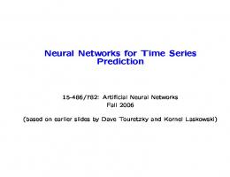
FIG. 2: Return map for a quasiperiodic (left) and chaotic(right) time series used for training a perceptron as described in the text

When trying to find the couplings wT by inverting the set of Eq. 1, it turns out that even professional computer routines often fail to perform the required matrix inversion: the patterns are almost linearly dependent. Some explanation for that can be found from Eq. 5. For small A, the tanh in Eq. 5 can be approximated by its argument and one can easily show that st+2 = −st + 2 cos(2πq/N )st+1 . Therefore, any window of the sequence can be written as a linear combination of two basis vectors. In case we expand the tanh in Eq. 5 up to the ρ’s term, one can Pρ−1 show that theP form of st+m is given by st+m (ρ) = k=0 B2k+1 (cos(2πq/N (2k + 1)) − sin(2πq/N (2k + 1))), since cos(x)2ρ+1 = C2k+1 cos((2k + 1)x) where Ck and Bk are constants. On one hand, as long as ρ is less than the window size N , the inputs are linearly dependent and Eq. 5 cannot be inverted. On the other hand, the power expansion of the tanh indicates that Bρ drops exponentialy with ρ. Thus, the linear dependence of the N -dimensional inputs is lifted only by the ρ = N + 1 term in the expansion which decreases exponentially as N increases. This is the source for the ill-conditioned problem of inverting Eq. 5. Hence, in particular for large dimensions N , batch learning does not work well for quasiperiodic time series generated by a teacher perceptron. How does this scenario show up in an on–line training algorithm for a continuous perceptron? If a quasiperiodic sequence is learned step by step using gradient descent to update the weights, without iterating previous steps, ∆wiS =

N X η wjS st−j (st − g(h)) · g ′ (h) · st−i with h = β N j=1

(6)

we find two time scales (time = number of training steps): (i) A fast one increasing the overlap between teacher and student to a value which is still far away from perfect agreement, R = 1 and QS = QT . During this phase, the training error goes down to nearly zero. (ii) A slow one further increasing the overlap and still decreasing the training error. Since the second time scale is usually several orders of magnitude larger than the first one, we could not observe R = 1 within our numerical simulations. Although there is a mathematical theorem on stochastic optimization which seems to guarantee convergence to zero training error (2) [10], which implies full overlap R = 1 with QS = QT , our on–line algorithm cannot gain much information about the teacher network, at least within practical times. This is completely different for a chaotic time series generated by a corresponding teacher network with g(x) = sin(β x) [9]. It turns out that learning the chaotic series works like learning random examples: After a number of training steps of the order of N the overlap R relaxes exponentially fast to perfect agreement between teacher and student, R = 1. The same behavior can be observed for the length QS of the student, which approaches exponentially fast to the length of the teacher. Here are some details of the numerical calculations: Our simulations were performed with the same (random) teacher weights for the quasiperiodic and the chaotic case. Furthermore, the random initialization of the student networks were identical. The settings differ only in the choice of the transfer-functions g(x). Return maps for the two sequences are shown in Fig. 2.

4 1

0.8

R

0.6

0.4

0.2

0

−0.2 0

5

10

α

15

20

25

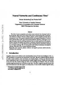
FIG. 3: Overlap R as a function of the fraction α = t/N of training examples. The upper curve shows the learning dynamic for the chaotic case, the lower one shows the two time scales for the training on the quasiperiodic series. Both settings start with the same initial overlap (R0 ≈ −0.16). At α ≈ 0.5 the dynamics of the quasiperiodic case enters the part with slow progress.

Starting with the same initial overlap, the students were trained according to Eq. (6) until they achieved a certain training error (ǫ = 0.008). In both cases this took about 25N learning steps, the network dimension was N = 50. After the training process however, the students ended up with completely different weight vectors. In case of the chaotic sequence, the student’s weights came close to the one of the teacher (R → 1,QS → QT ). In contrast, the student of the quasiperiodic sequence did not obtain much information about the teacher, and its weights remained nearly perpendicular to the teacher ones (R ≈ 0). The time evolution of the respective overlaps during training is shown in Fig. 3. One important question remains: How well can the student predict the time series? In order to evaluate the training success, we have defined a one-step-error in Eq. (2). Now we are interested in the long-term prediction of the students. Therefore, the student perceptrons have to act as sequence generators themselves, using their own output to complete the next input window. Starting from a window of the teacher’s sequence, i.e. (ot , ot−1 , ...ot−N +1 ) = (st , st−1 , ...st−N +1 ), the student’s prediction τ steps ahead is given by iterating Eq. (1) up to   N X (7) wjS ot+τ −j  ot+τ = g β j=1

The prediction error ǫ(τ ) is the average absolute deviation of this value with the respective item of the teacher’s sequence, t0 +T 1 X |st+τ − ot+τ | T →∞ T t=t +1

ǫ(τ ) = lim

(8)

0

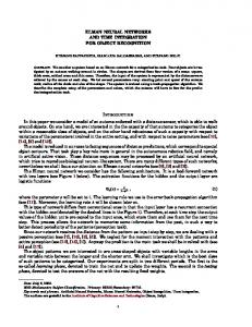
Note, that the average is performed by changing the initial time window. Again, t0 is used to indicate any time step of the stationary part of the sequence. To calculate ǫ(τ ) in the simulations, we have chosen T = N = 50. The result is shown in Fig. 4. The graph shows the prediction error as a function of the time interval over which the student makes predictions. Both curves coincide in the first value, which is equal to the training error at which learning was stopped. The student network which has been trained on the quasiperiodic sequence can predict it very well. The error increases linearly with the size of the interval, even predicting 25N steps ahead yields an error of less than 5% of the total possible range. On the other side, the student trained on the chaotic sequence cannot make long-term predictions. The prediction error increases exponentially with time until it is of the order of random guessing.

5 1.2

1

0.8

ε

0.6

0.4

0.2

0 0

10

20

α

30

40

50

FIG. 4: Prediction error as a function of time steps ahead (measured in multiples of N : α = τ /N ), for the quasiperiodic (lower) and the chaotic (upper) series.

Of course, if the student would reproduce the series perfectly, it would also predict it without errors. But since we stop our algorithm when the training error is close but not identical to zero, we achieve two different states: For the quasiperiodic sequence the weight vector of the student recovers the main Fourier component of the teacher which reproduces the sequences reasonably well. There remains a large space of weight vectors which can generate the same sequence. For the chaotic sequence, however, all the weights of the students come extremely close to the ones of the teacher; but due to sensitivity to model parameters, any prediction of the sequence is impossible. All of our results stem from numerical simulations. We find that the quantitative details of our results strongly depend on the parameters of our model. Hence we did not succeed to derive quantitative results about scaling of learning times with system size N or the Ljuapunov exponent as a function of the fractal dimension of the chaotic time series. In summary we obtain the following result: (i) A network trained on a quasiperiodic sequence does not obtain much information about the teacher network which generated the sequence. But the network can predict this sequence over many (of the order of N ) steps ahead. (ii) A network trained on a chaotic sequence, however, obtains almost complete knowledge about the teacher network. But due to the chaotic nature of the sequence, this network cannot make reasonable predictions.

[1] A. Weigand and N. S. Gershenfeld: Time Series Prediction, Santa Fe, (Addison Wesley, 1994) [2] Hertz, J. and Krogh, A., and Palmer, R.G.: Introduction to the Theory of Neural Computation, (Addison Wesley, Redwood City, 1991) [3] Engel, A. and Van den Broek, C.: Statistical Mechanics of Learning, (Cambridge University Press, 2001) [4] M. Biehl and N. Caticha: Statistical Mechanics of On-line Learning and Generalization, The Handbook of Brain Theory and Neural Networks, ed. by M. A. Arbib (MIT Press, Berlin 2001) [5] E. Eisenstein and I. Kanter and D.A. Kessler and W. Kinzel: Generation and Prediction of Time Series by a Neural Network, Phys. Rev. Letters 74, 6-9 (1995) [6] I. Kanter and D.A. Kessler and A. Priel and E. Eisenstein: Analytical Study of Time Series Generation by Feed-Forward Networks, Phys. Rev. Lett. 75, 2614-2617 (1995) [7] M. Schr¨ oder and W. Kinzel: Limit cycles of a perceptron, J. Phys. A 31, 9131-9147 (1998) [8] L. Ein-Dor and I. Kanter: Time Series Generation by Multi-layer networks, Phys. Rev. E 57, 6564 (1998) [9] A. Priel and I. Kanter: Robust chaos generation by a perceptron, Europhys. Lett. 51, 244-250 (2000) [10] C. M. Bishop: Neural Networks for Pattern Recognition (Oxford University Press, New York 1995)