Learning Ground CP-logic Theories by means of Bayesian Network

Learning Ground CP-logic Theories by means of Bayesian Network Techniques Wannes Meert, Jan Struyf and Hendrik Blockeel Department of Computer Science, Katholieke Universiteit Leuven, Celestijnenlaan 200A, 3001 Leuven, Belgium, {wannes.meert, jan.struyf, hendrik.blockeel}@cs.kuleuven.be

Abstract. Causal relationships are present in many application domains. CP-logic is a probabilistic modeling language that is especially designed to express such relationships. This paper investigates the learning of CP-theories from examples, and focusses on structure learning. The proposed approach is based on a transformation between CP-logic theories and Bayesian networks, that is, the method applies Bayesian network learning techniques to learn a CP-theory in the form of an equivalent Bayesian network. We propose a constrained refinement operator for such networks that guarantees equivalence to a valid CP-theory. We experimentally compare our method to a standard method for learning Bayesian networks. This shows that CP-theories can be learned more efficiently than Bayesian networks given that causal relationships are present in the domain.

1

Introduction

Bayesian networks have earned a good reputation for modeling complex problems involving uncertain knowledge. This success seems to be at least in part due to the causal interpretation that can be given to such networks. Although it is theoretically impossible to infer all causal relationships from a typical data set, it still seems useful to try to approximate them by means of learning, mainly because causal information tells you just enough about the (expected) behavior of a process, while allowing irrelevant details to be ignored [1]. This causality is, however, not present in the formal semantics of Bayesian networks (although there is some work on causal Bayesian networks [2]). Causal Probabilistic logic (CP-logic), on the other hand, is a probabilistic modeling language with causality at the heart of its fundamental construct. Because CP-logic focusses on causal information, in a sense, it allows a more fine-grained and flexible representation than Bayesian networks [1]. This results in a smaller number of parameters and easy to read theories. This is not only useful for human experts, but also for automated model building algorithms. Indeed, a lot of effort goes into obtaining the structure of the model and the numerical parameters that are needed to fully quantify it. For example, in a Bayesian network, a binary variable with n parents will require 2n parameters to be defined. For a large value of n this is not only a heavy task for a human

expert but it also requires sufficiently large data sets to accurately learn all these parameters [3, 4]. A CP-logic theory (CP-theory), on the other hand, has only one parameter for every cause. There is already some work on learning a subset of CP-logic by Riguzzi [5]1 . This subset was extended by Blockeel and Meert [6] by using a conversion to Bayesian networks. The latter method offers the possibility to adapt some of the many methods and optimizations available for Bayesian networks to learn a CP-theory. Where Blockeel and Meert [6] mainly focus on parameter learning, in this paper, we offer a practical method for learning the structure of a large subset of CP-theories by using this conversion to Bayesian networks. We start this article with a brief introduction to CP-logic in Section 2. In Section 3, we explain the link with Bayesian networks and how to convert a CP-theory to a Bayesian network. Finally, we adapt some Bayesian learning algorithms to learn a CP-theory from data in Section 4 and Section 5.

2

Intuitions about CP-logic

We briefly introduce CP-logic. A more formal description can be found in [1]. A CP-theory can be seen as a set of if-then rules of the following form: (h1 : α1 ) ∨ (h2 : α2 ) ∨ . . . ∨ (hn : αn ) ← b1 , b2 , . . . , bm . with P hi atoms and bi literals in the logical sense, all causal probabilities αi ∈ [0, 1], n and i=1 αi ≤ 1. We call the set of all (hi : αi ) the head of the rule, and the set of all bi the body. If the head contains only one atom h : 1, we may write it as h. Each of these rules has several possible conclusions (head), each of which has a certain probability (αi ) assigned to it. The rule makes exactly one of the conclusions true with the associated probability. For instance, (spaghetti : 0.5) ∨ (steak : 0.5) ← shops(john). expresses that if John goes shopping, he buys spaghetti or steak for dinner each with 50% chance. Multiple rules in a CP-theory may lead to the same conclusions. Take, for instance, the following CP-theory (spaghetti : 0.5) ∨ (steak : 0.5) ← shops(john). (spaghetti : 0.3) ∨ (f ish : 0.7) ← shops(mary). which expresses that if John goes shopping he buys spaghetti or steak for dinner and if his girlfriend Mary goes shopping, she buys spaghetti or fish. The numbers associated with the different meals indicate the probability that the event mentioned in the rule body causes that type of dinner to be bought. If both go 1

Note that CP-logic theories and LPADs (Logic Programs with Annotated Disjuctions) are equivalent. The research about LPADs has evolved into CP-logic.

shopping it is possible that they buy both steak and fish, in that case they can choose what they will have for dinner. It is part of the semantics of CP-logic that each rule independently of all other rules makes one of its head atoms true when triggered. CP-logic is therefore particularly suitable for describing models that contain a number of independent stochastic events or causal processes. Consequently, learning a CP-theory amounts to discovering the causal structure of possibly complex processes. It may be tempting to interpret the parameters as the conditional probability of a head atom given the body, e.g., P r(spaghetti|shops(mary)) = 0.3, but this is incorrect. The conditional probability that spaghetti is bought, given that Mary went shopping, is higher than 0.3, because there is a second possible cause, namely that John also bought spaghetti. To compute this conditional probability, we need information on the probability that John went shopping. For instance, with shops(john) : 0.2. shops(mary) : 0.9. (spaghetti : 0.5) ∨ (steak : 0.5) ← shops(john). (spaghetti : 0.3) ∨ (f ish : 0.7) ← shops(mary). we can say that P r(spaghetti|shops(mary)) = 0.3 + 0.2 · 0.5 · 0.7 = 0.37 : Mary buys spaghetti with probability 0.3, but there is also a probability of 0.2 that John went to the shop, and hence a probability of 0.2 · 0.5 · 0.7 that spaghetti is bought by John (0.2 · 0.5) and not by Mary (0.7). Thus, for head atoms that occur in multiple rules, the mathematical relationship between the CP-theory parameters and conditional probabilities is somewhat complex, but it is not unintuitive. The meaning of the probabilities in the rules is quite simple: they reflect the probability that the body causes the head to become true. This is different from the conditional probability that the head is true given the body, but among the two, the former is the more natural one to express. Indeed, the former is local knowledge: an expert can estimate the probability that shops(mary) causes spaghetti without considering any other possible causes for spaghetti. To infer P r(spaghetti|shops(mary)), we need global knowledge: we need to know all possible causes for spaghetti, the probability of them occurring, and how they interact with shops(mary). The fact that the parameters in a CP-theory are local makes it impossible to estimate them directly from the data as can be done in Bayesian networks. In Section 3, we will see that CP-theory parameters can be mapped to Bayesian network parameters by introducing unobserved nodes.

3

Converting a CP-logic Theory to a Bayesian Network

Blockeel and Meert [6] show that any CP-theory that is non-recursive and has a finite Herbrand universe can be converted into a Bayesian network such that the

CP-theory parameters appear in the network’s CPTs2 . All other CPT entries are either 0.0 or 1.0. In this section, we explain this conversion. We only consider ground CP-theories, so a non-ground CP-theory must be grounded first. Based on such a CP-theory we construct a Bayesian network. The structure can be created in three steps: 1. For every literal in the CP-theory, a Boolean variable is created in the Bayesian network. This is a so-called literal variable and is represented by a literal node in the network. 2. For every rule in the CP-theory, a choice variable is created in the Bayesian network. This variable can take k + 1 values, where k is the number of atoms in the head. It is represented by a choice node in the network. 3. If an atom is in the head of a rule, an edge is created from its corresponding choice node towards the atom’s node. If a literal is in the body of a rule, an edge is created from the literal node towards the rule’s choice node. For the CPTs there are two cases: 1. The CPT of a choice variable (e.g., Fig. 1 CPT for C3): such a variable can take k + 1 values with k the number of atoms in the head. The variable has the value i if the ith atom from the head is chosen by the probabilistic process. If none is chosen (in case the probabilities do not sum up to one) then the variable has the value 0. The probability that the variable takes a particular value if the body is true, is the causal probability given in the rule of the CP-theory. If the body is not true, the probability that the choice variable takes the value 0 is 1.0 and all the other values have probability 0.0. Note, that a body may contain negative literals. 2. The CPT of a literal variable (e.g., Fig. 1 CPT for spaghetti) is structured differently. If the choice variable of a rule in which the atom is in the head has as value the position of that atom in the head, then it will be true with probability 1.0, otherwise it will be false. As an example, the conversion of the shopping example to a Bayesian network is depicted in Fig. 1. It can be noted that this structure resembles noisy-or structures as introduced by Pearl [7]. This is partly due to the fact that CPlogic uses the principle of independent causation, which is similar to the principle of independence of causal influence (ICI). ICI models are a family of Bayesian network models used for classification tasks with large numbers of attributes. So, a simple CP-theory can be used as an ICI classifier. Since we can convert a CP-theory to a specific type of Bayesian network, we have two different representations for the same CP-theory. To differentiate between them we will name them. All the possible CP-theories expressed in the CP-logic syntax and semantics will be called the CP-logic space. The Bayesian networks resulting from the conversion are part of what we will call the Bayesian network space. So, this is the space of all the possible Bayesian networks that are equivalent to a valid CP-theory. 2

CPTs are Conditional Probability Tables as known for Bayesian Networks. Note that Conditional Probability is not the same as Causal Probability (Section 2).

C1

C2

shops(john)

shops(mary)

C3

steak

C4

spaghetti

fish

(a) Bayesian network

C1 0 1

0.8 0.2

john(shops) T F C3 0 1 2

C1=1 1 0

john(shops) 0 0.5 0.5

spaghetti T F

other 0 1

other 1 0 0

C3=1 or C4=1 1 0

other 0 1

(b) CPTs for some nodes of (a)

Fig. 1. Conversion from a CP-theory to a Bayesian network.

4

Parameter Learning

Once this equivalent Bayesian network is created we can use known methods for learning Bayesian networks to learn the parameters of the network and thus also the CP-theory parameters. It is, however, necessary to impose constraints on the CPTs in order to keep the network equivalent to a valid CP-theory. As input we use a multi-set of tuples and each tuple indicates the truth value (true or false) of each literal in the domain. The choice variables in the Bayesian network are not present in our domain, therefore the network is not fully observable. This is solved by using an EMalgorithm for learning the parameters [8]. Because we use an EM-algorithm, the missing values are allowed in the input data. While the choice variables introduce unobserved variables, which is a disadvantage, the structure of the CP-theory gives extra information about the structure of the CPTs, which can make the learning more efficient. Many of the parameters are 0.0 or 1.0 (Fig. 1). These values are known in advance and don’t need to be learned, to the contrary, they can be used to speed up the EM-algorithm. Only the values that are not 0.0 or 1.0 have to be learned; these are the original parameters of the CP-theory. To force the CPTs to have ones and zeros in the right positions after learning, it suffices to initialize these parameters with 0.0 or 1.0. The Bayesian update rule in the expectation-step can only update values strictly between 0 and 1. Since the prior probability is set, e.g., to 0.0 the posterior probability is also 0.0. So, a standard EM parameter learning algorithm for Bayesian networks learns the correct parameters for our CP-theory. The method outlined above is a simple application of the EM-algorithm. This can, however, be further optimized. The CPTs that only contain probabilities 0.0 or 1.0 are actually not describing a probability distribution but a functional dependency. These are rather functions where there is just one result and it is

calculated based on the input, not a set of results with each a probability. Since this network contains many functional dependencies, extra optimizations can be incorporated into the algorithm. For example, an optimization specific for noisy-or implementations is given by Vomlel [9].

5

Structure Learning

Besides learning the parameters, we also need to learn the structure of a CPtheory. This involves a search over possible CP-theories, which can be done either in CP-logic space or in Bayesian network space. In the previous section, we learned the parameters in the Bayesian network space. Here we consider learning the structure also in the Bayesian network space. This avoids the conversion each time the algorithm investigates a new candidate structure. An important constraint when searching the Bayesian network space for possible structures is that every Bayesian network must have a valid mapping to a CP-theory. The learning algorithm that we propose is based on the structural EMalgorithm (SEM) introduced by Friedman [10]. This is a greedy search algorithm, outlined in Table 1 for both the CP-logic space and the Bayesian network space. The refinement function returns a Bayesian network in the neighborhood of the current network. The eval function evaluates the new network. CPtheory := ∅ while CPtheory is not good enough: S := refinements(CPtheory) CPtheory := argmaxL∈S eval(L) return CPtheory

BN := initial Bayesian net while BN is not good enough: S := refinements(BN) BN := argmaxL∈S eval(L) return CPtheory(BN)

Table 1. Greedy SEM algorithm to learn the structure of a CP-theory.

5.1

Evaluation Function

The evaluation function is typically based on the likelihood of the data given the candidate model after learning the parameters. In this case, the Bayesian Information Criterion (BIC) is used [8]. The main advantage of this measure is its modularity. Every node in the network has its own local score and the sum of these scores is the total score. In this way we only have to recalculate the score of the part of the new structure that has changed with respect to the previous structure to see if it is better or not. As the BIC function prefers smaller networks, our algorithm prefers smaller CP-theories. 5.2

Refinement Function

The refinement operators are similar to those in the SEM-algorithm and perform a greedy hill-climbing neighborhood search. More concrete, the SEM operators

add, delete or invert one edge of the current network. Our algorithm takes a similar approach, but takes into account the specific structure of a Bayesian network that represents a CP-theory. As we have seen previously, the choice nodes represent the rules in the CPtheory and the edges are defined by the literals in the head and the body. Based on this we introduce the following constraints on possible networks. – – – –

Only edges between a literal node and a choice node are allowed. A literal node has at least one incoming edge. A literal node is a Boolean variable. A choice node is a variable that can take values from 0 to k with k number of atoms in the head. – The CPT of aliteral node contains only 0 or 1, based on the structure of CP-theory. – The CPT of a choice node has in the column where the body is true CP-theory parameters. In all the other columns the choice node takes value 0 with probability 1.

the the the the

These constraints guarantee that the resulting Bayesian networks are equivalent to a CP-theory and all the entries in the CPTs except the CP-theory parameters are 1.0 or 0.0. There are three possible actions to find a network in the neighborhood of the current one: 1) adding a relation between two literals, 2) deleting a relation or 3) inverting a relation. A relation between two literals in this context means that there is a rule in the theory that has one of the literals in the head and the other one in the body. Translated to the Bayesian network space, this is the existence of a choice node with an incoming edge from one of the literals and an outgoing edge to the other literal. Fig. 2 gives an overview of the different refinement types, a detailed description follows next. Deleting a Relation Deleting an edge corresponds to deleting a literal from a rule. This can be done by removing the edge between a literal node and a choice node. If the choice node has no outgoing edges after the removal of the edge, the choice node itself is also removed. A graphical example can be seen in Fig. 2.a. In the first step in the figure it is shown that a rule can be eliminated by removing a choice node and its edges. The second step removes a literal from the body of a rule by eliminating an incoming edge of the choice node that represents that rule. Adding a Relation Adding an edge between a choice node and a literal node is the same as adding a literal to an existing rule in the CP-theory. To add an atom to the head of a rule, an edge is created departing from the choice node representing that rule to the literal node representing the added atom. Adding a literal to the body of a rule is accomplished by adding an edge from the literal node to

C1

C1 del

X

C2

C3

X

C1 del

C2

Y

Y

x : α1 . y : α2 ← x. y : α3 .

x : α1 . y : α2 ← x.

C1

C2

X

X

Y

C2

Y

x : α1 . y : α2 .

C1 inv

X

C4

Z

C2

C5

Y

x : α1 . y : α21 ∨ z : α22 ← x.

a

C3

Z

x : α1 . x : α2 ← y. x : α3 ← z. y : α4 . z : α5 .

b c

C1

C2

C3

C1

C2

C3

add X

Y

Z

C1

C2

C3

add X

Y

Z

X

Y

C4

x : α1 . y : α2 . z : α3 .

x : α1 . y : α2 ← x. z : α3 .

C1

C2

add

x : α1 . y : α2 ← x. z : α3 . y : α4 ← ¬x.

Z

X

Y

C4

C3

Z

x : α1 . y : α2 ← x. z : α3 . y : α41 ∨ z : α42 ← ¬x.

Fig. 2. Examples of the refinement operator. The dotted arrow represents a rule where that particular literal is negated in the body of the rule.

the choice node. To create a new rule, a new choice node must be created with incoming and outgoing edges based on the literals that are present in the new rule. In the first step of Fig. 2.c, a literal is added to the body of the second rule. The equivalent step in the Bayesian network space is adding the incoming edge to the choice node departing from the literal node, corresponding respectively to the rule and the literal in the CP-theory. This simple addition of a literal to the body of a rule, is a too simplistic step typically resulting in a CP-theory with a low likelihood. Before introducing an extension that will overcome this problem, we will first explain in more detail why this is necessary. In a CP-theory a literal can become only true if it has a reason to become true, i.e., if the body of a rule where it is in the head is true. Suppose that a literal is only present in one rule as for example in the second rule of the CP-theory in Fig. 2.c (y : α2 ). The literal y can become true independent of the other literals (because the body is always true). After adding a literal to the body of that rule (x after step 1), the head can only become true if the body (x) is true. Suppose that in the target theory, y can also be true if x is false (y has multiple causes), the current theory will then have a low likelihood, because the data will contain cases where y is true and x false. The new body of the rule constraints the head too much, but, on the other hand, we may want to have a relation between the head and the new body as one of the possible causes. To check if the new body is the cause of the head, but not the only one, we perform a lookahead step. When the likelihood is very low after adding a literal

to the body of a rule, we add an additional new rule. This rule is identical to the previous one with the exception that the newly added literal is negated. This new rule covers the causes not yet discovered, be it in a rudimentary way. In a subsequent step the algorithm can find another cause for the head and add this to the rule with the negated literal, possibly even removing this negated literal in a future step. This addition of this new rule is illustrated in step 2 of Fig. 2.c. Inverting a Rule With inverting we mean switching the direction of the causation. It is sometimes possible that the algorithm learns the first relationship between literals with the wrong direction of causation. Because the algorithm builds further upon already learned networks, the incorrect direction of the causation may persist when subsequent relationships are added. And although the initial relationship had, by coincidence, a good likelihood, the following steps are not optimal. This operator can detect such situations and reverse them. The direction of causation is defined in a rule in the CP-theory from the body towards the head. To invert this direction we must somehow switch head and body. Consequently the edges of the corresponding choice node have to be inverted. It is, however, not possible to just invert all the edges. If a rule has multiple consequences, it is necessary to split up the node into a different choice node for every consequence in the rule. This is because the consequents in the head are a disjunction and only reversing the direction of the edges would convert this disjunction into a conjunction, which is incorrect. Therefore, we create a separate rule for each consequent (see Fig. 2.b). The same reasoning applies for rules with multiple conditions in the body.

6

Experiments

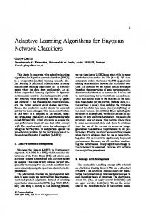
As experiment we compare the performance of our algorithm to learn a CPtheory with the SEM algorithm to learn a Bayesian network (no unobserved variables). The SEM algorithm used can be found in the Structure Learning Package [11], which is an extension to the Bayesian Network Toolbox [12] for Matlab. We construct the input data by sampling interpretations from the CP-theory described in the shopping example (Fig. 1). The test set is fixed and consists of 1000 examples. In each trial, we sample a training set of a given size. The learning algorithms train on this sample, and the resulting models (CP-theory or Bayesian network) are tested on the fixed test set. We report, for each method and training set size, the test set log likelihood averaged over at least 10 trials. Fig. 3 presents the results. The thick lines are the mean log likelihood of both methods and the dashed lines represent 90% confidence intervals for the mean. The graph also plots the minimum and maximum log likelihood measured for both methods over all trials. The figure shows the results of the CP-logic structure learning algorithm and the SEM structure learning for Bayesian networks. For the two methods, the

-600

log likelihood of test data

-800

-1000

-1200

-1400

CP-theory 90% confidence interval min max Bayesian Network 90% confidence interval min max

-1600

-1800

-2000

0

100

200 300 500 400 Number of interpretations in training set

600

Fig. 3. Comparing structure learning of CP-theories and Bayesian Networks.

average log likelihood converges, but the learned CP-logic theory has on average a better log likelihood than the Bayesian network. This is because the Bayesian network has difficulties to represent a causal structure like the shopping example. It is possible that the log likelihood of the Bayesian network comes close to the log likelihood of the CP-theory as can be seen for the cases where there are 100 and 500 examples in the training set. This is however an exception as the SEM algorithm prefers a small network, and representing the target theory requires many edges (and parameters) if no additional hidden variables are introduced. The SEM algorithm seldom finds such a network, but if it does, it raises the average likelihood a little bit. Causality imposes a strong connection between the literals’ truth values in the data set. In this case the data set is derived from a causal process and in CP-logic this can be described with a small theory. A Bayesian network, on the other hand, requires many edges and parameters to represent such a theory. Therefore, it is more useful to search for a CP-theory in this case. When an incorrect causal relationship is inferred from the data set, this can result in a theory with a very low likelihood because of the same reasons. Suppose that in a given training set a literal y is only true when the literal x is true, this may result in learning this causal relation. If this relationship is not present in the target theory, the test set will also contain cases where y is true and x is false. Such a case is not covered by the learned structure and results in an extremely low likelihood as can be seen from the minima in the graph. These, however, are exceptions and therefore the average is still good. Running the algorithm multiple times starting from different initial theories often solves this.

Because of this strong causal connection, when learning from a small training set, the quality of the training set is important for learning a correct CP-theory. This can be seen when looking at the maxima in the graph; even when learning from small training sets, the algorithm can learn a good theory (the best log likelihoods in our experiments correspond to cases where the algorithm learned the correct structure of the target theory). When the training set is large enough the algorithm finds a good theory for every training set.

7

Conclusions and Future Work

We proposed a method for learning the structure of a ground CP-theory. It is based on existing methods for learning Bayesian networks, but uses refinement operators specific to CP-logic. The main advantage of this approach is the possibility to reuse some of the large amount of the research available in the Bayesian networks literature [13, 14]. We have compared structure learning for CP-theories to structure learning for Bayesian networks. CP-theories better approximate the target theory than Bayesian networks if it contains causal relationships. Compared to CP-theories, standard Bayesian network algorithms need to learn more edges and parameters in the corresponding CPTs to approximate such a theory, and this is detrimental to the efficiency of the learning. We consider the following directions for further work. We plan to extend the experimental evaluation. First, it would be interesting to compare our method for learning CP-theories to a method for learning Bayesian networks that allows the introduction of hidden variables; our translation of CP-theories also uses these for the choice nodes. Second, there are specific techniques for representing causality in Bayesian networks [2]. It would be interesting to compare to such work. Our current evaluation is on one artificial domain. We plan to evaluate the method on more data sets and in real world applications. Finally, the present paper considers ground CP-theories. Further work will address learning of CPtheories with abstract rules (i.e., rules with variables).

Acknowledgments Wannes Meert is supported by the Institute for the Promotion of Innovation by Science and Technology in Flanders (IWT-Vlaanderen). Jan Struyf and Hendrik Blockeel are post-doctoral fellows of the Research Foundation - Flanders (FWO-Vlaanderen). Research supported by project GOA/2003/08 (B0516) on Inductive Knowledge Bases.

References 1. Vennekens, J., Denecker, M., Bruynooghe, M.: Extending the role of causality in probabilistic modeling. In: Proceedings of the 11th International Workshop on Non-monotonic Reasoning. (2006) 183–190

2. Pearl, J.: Causality: Models, Reasoning, and Inference. Cambridge University Press (2000) 3. Onisko, A., Druzdzel, M.J., Wasylu, H.: Learning Bayesian network parameters from small data sets: Application of Noisy-OR gates. In: Working Notes of the Workshop on Bayesian and Causal Networks: From Inference to Data Mining, 12th European Conference on Artificial Intelligence (ECAI-2000), Berlin, Germany (22 August 2000) 4. Friedman, N., Goldszmidt, M.: Building classifiers using Bayesian networks. In: AAAI/IAAI, Vol. 2. (1996) 1277–1284 5. Riguzzi, F.: Learning logic programs with annotated disjunctions. In Srinivasan, A., King, R., eds.: 14th Internation Conference on Inductive Logic Programming (ILP2004), Porto, Heidelberg, Germany, Springer Verlag (September 2004) 270– 287 6. Blockeel, H., Meert, W.: Towards learning non-recursive LPADs by transforming them into Bayesian networks. In Muggleton, S., Otero, R., eds.: International Conference on Inductive Logic Programming. (2006) 7. Pearl, J.: Probabilistic reasoning in intelligent systems: Networks of plausible inference. Morgan Kaufmann, San Francisco (1988) 8. Neapolitan, R.: Learning Bayesian Networks. Prentice Hall, Upper Saddle River, NJ, USA (2003) 9. Vomlel, J.: Noisy-or classifier. International Journal of Intelligent Systems 21(3) (2006) 381–398 10. Friedman, N.: Learning belief networks in the presence of missing values and hidden variables. In: Proc. 14th International Conference on Machine Learning, Morgan Kaufmann (1997) 125–133 11. Leray, P., Francois, O.: BNT structure learning package: Documentation and experiments. Technical report, Laboratoire PSI (2004) 12. Murphy, K.P.: Bayesian network toolbox, http://bnt.sourceforge.net/ 13. Heckerman, D., Geiger, D., Chickering, D.M.: Learning Bayesian networks: The combination of knowledge and statistical data. In: Proc. 10th Conf. Uncertainty in Artificial Intelligence, San Francisco, CA, Morgan Kaufmann Publishers (1994) 293–301 14. Jensen, F.V.: Introduction to Bayesian Networks. Springer-Verlag New York, Inc., Secaucus, NJ, USA (1996)