Learning in non-stationary Partially Observable Markov ... - McGill CS

Learning in non-stationary Partially Observable Markov Decision Processes Robin JAULMES, Joelle PINEAU, Doina PRECUP McGill University, School of Computer Science, 3480 University St., Montreal, QC, Canada, H3A2A7

Abstract. We study the problem of finding an optimal policy for a Partially Observable Markov Decision Process (POMDP) when the model is not perfectly known and may change over time. We present the algorithm MEDUSA+, which incrementally improves a POMDP model using selected queries, while still optimizing the reward. Empirical results show the response of the algorithm to changes in the parameters of a model: the changes are learned quickly and the agent still accumulates high reward throughout the process.

1

Introduction

Partially Observable Markov Decision Processes (POMDPs) are a well-studied framework for sequential decision-making in partially observable domains (Kaelbling et al, 1995) . Many recent algorithms have been proposed for doing efficient planning in POMDPs (Pineau et al. 2003; Poupart & Boutilier 2005; Vlassis et al. 2004). However most of these rely crucially on having a known and stable model of the environment. On the other hand, the experience-based approaches (McCallum, 1996; Brafman and Shani, 2005; Singh et al. 2004) also need a stationary model. They also require very large amounts of data, which would be hard to obtain in a realistic application. In many applications it is relatively easy to provide a rough model, but much harder to provide an exact one. Furthermore, because the model may be experiencing some variations in time, we would like to be able to use experimentation to improve our initial model. The overall goal of this work is to investigate POMDP approaches which can combine a partial model of the environment with direct experimentation, in order to produce solutions that are robust to model uncertainty and evolution, while scaling to large domains. To do that, we will assume that uncertainty is part of the model and design our agent to take it into account when making decisions. The model will then be updated based on every new experience. The technique we propose in this paper is an algorithm called MEDUSA+, which is an improvement of the MEDUSA algorithm we presented in Jaulmes et al., 2005. It is based on the idea of active learning (Cohn et al. 1996), which is a well-known technique in machine learning for classification tasks with sparsely labelled data. In active learning the goal is to select which examples should be labelled by considering the expected information gain. As detailed by Anderson and Moore (2005), these ideas extend nicely to dynamical systems such as HMMs. We will assume in the present work the availability of an oracle that can provide the agent with exact information about the current state, upon request. While the agent

experiments with the environment, it can ask for a query in order to obtain state information, when this is deemed necessary. The exact state information is used only to improve the model, not in the action selection process, which means that we may have a delay between the query request and the query processing. This is a realistic assumption, since in a lot of realistic applications (robotics, speech management), it is sometimes easy to determine the exact states we went through after the experimentation has taken place. The model uncertainty is represented using a Dirichlet distribution over all possible models, in a method inspired from Dearden et al., 1999 and its parameters are updated whenever new experience is acquired. They also decay with time, so recent experience has more weight than old experience, a useful feature for non-stationary POMDPs. The paper is structured as follows. In Section 2 we review the basic POMDP framework. Section 3 describes our algorithm MEDUSA+, and outlines modifications that we made compared to MEDUSA. Section 4 shows the theoretical properties of MEDUSA+. Section 5 shows the performance of MEDUSA+ on standard POMDP domains. In Section 6 we discuss the relationship of our approach to related work and our conclusion is in Section 7.

2

Partially Observable Markov Decision Processes

We assume the standard POMDP formulation (Kaelbling et al., 1998); namely, a POMDP consists of a discrete and finite set of states S, of actions A and of observations Z. It has a } = {p(s 0 0 transition probabilities {Ps,s 0 t+1 = s |st = s, st = a)}, ∀s ∈ S, ∀a ∈ A, ∀s ∈ S and a observation probabilities {Os,z } = {p(zt = z|st = s, at−1 = a)}, ∀z ∈ Z, ∀s ∈ S, ∀a ∈ A. It also has a discount factor γ ∈ (0, 1] and a reward function R : S × A × S × Z → IR, such that R(st , at , st+1 , zt+1 ) is the immediate reward for the corresponding transition. At each time step, the agent is in an unknown state st ∈ S. It executes an action at ∈ A, arriving in an unknown state st+1 ∈ S and getting an observation zt+1 ∈ Z. Agents using POMDP planning algorithms typically keep track of the belief state b ∈ IR|S| , which is a probability distribution over all states given the history experienced so far. A policy is a function that associates an action to each possible belief state. Solving a POMDP means finding the policy that maximizes the expected discounted return T E(∑t=1 γ t R(st , at , st+1 , zt+1 )). While finding an exact solution to a POMDP is computationally intractable, many methods exist for finding approximate solutions. In this paper, we use a point-based algorithm (Pineau et al. 2003), in order to compute POMDP solutions. However, the algorithms that we propose can be used with other approximation methods. We assume the reward function is known, since it is directly linked to the task that a } and {Oa }. These probwe want the agent to execute, and we focus on learning {Ps,s 0 s,z ability distributions are typically harder to specify correctly by hand, especially in real applications. They may also be changing over time. For instance in robotics, the sensor noise and motion error are often unknown and may also vary with the amount of light, the wetness of the floor, or other parameters that it may not know in advance. To learn the transition and observation models, we assume that our agent has the ability to ask a

query that will correctly identify the current state 1 . This is a strong assumption, but not entirely unrealistic. In fact, in many tasks it is possible (but very costly) to have access to the full state information; it usually requires asking a human to label the state. As a result, clearly we want the agent to make as few queries as possible.

3

The MEDUSA+ algorithm

In this section we describe the MEDUSA+ algorithm. Its main idea is to represent the model uncertainty with a Dirichlet distribution over possible models, and to update directly the parameters of this distribution as new experience is acquired. To cope with non-stationarity, we decay the parameters as time goes. Furthermore, MEDUSA+ uses queries more efficiently, through the use of the alternate belief and of non-query learning. This approach scales nicely: we need one Dirichlet parameter for each uncertain POMDP parameter, but the size of the underlying POMDP representation remains unchanged, which means that the complexity of the planning problem does not increase. However this approach requires the agent to repeatedly sample POMDPs from the Dirichlet distribution and solve them, before deciding on the next query. 3.1

Dirichlet Distributions

Consider a N-dimensional multinomial distribution with parameters (θ1 , . . . θN ). A Dirichlet distribution is a probabilistic distribution over these parameters. The Dirichlet itself is parameterized by hyper-parameters (α1 , . . . αN ). The likelihood of the multinomial parameters is defined by: p(θ1 . . . θN |D) =

α −1

∏Ni=1 θi i Z(D)

, where Z(D) =

∏Ni=1 Γ(αi ) Γ(∑Ni=1 αi )

The maximum likelihood multinomial parameters θ∗1 . . . θ∗N can be computed, based on this formula, as: αi θ∗i = N , ∀i = 1, . . . N ∑k=1 αk The Dirichlet distribution is convenient because its hyper-parameters can be updated directly from data. For example, if instance X = i is encountered, αi should be increased by 1. Also, we can sample from a Dirichlet distribution conveniently using Gamma distributions. In the context of POMDPs, model parameters are typically specified according to multinomial distributions. Therefore, we use a Dirichlet distribution to represent the uncertainty over these. We use Dirichlet distributions for each state-action pair where either the transition probabilities or the observation probabilities are uncertain. Note that instead of using increments of 1 we use a learning rate, λ, which measures the importance we want to give to one query. 1

We discuss later how the correctness assumption can be relaxed. For example we may not need to know the query result immediately

3.2

MEDUSA

The name MEDUSA comes from ”Markovian Exploration with Decision based on the Use of Sampled models Algorithm”. We present here briefly the algorithm as it was described in Jaulmes et al., 2005. MEDUSA has the following setup: first, our agent samples a number of POMDP models according to the current Dirichlet distribution. The agent then computes the optimal policy for each of these models, and at each time step one of those is chosen with a probability that depends on the weights these models have in the current Dirichlet distribution. This allows us to obtain reasonable performance throughout the active learning process: the quality of the sampled models will be linked to the quality of the actions chosen. This also allows the agent to focus the active learning in regions of the state space most often visited by good policies. Note that with MEDUSA we need not specify a separate Dirichlet parameter for each unknown POMDP parameter. It is often the case that a small number of hyperparameters suffice to characterize the model uncertainty. For example, noise in the sensors may be highly correlated over all states and therefore we could use a single set of hyper-parameters for all states. In this setup, the corresponding hyper-parameter would be updated whenever action a is taken and observation z is received, regardless of the state.2 This results in a very expressive framework to represent model uncertainty. As we showed our previous work, we can vary the number of hyper-parameters to trade-off the number of queries versus model accuracy and performance. Each time an action is made and an observation is received, the agent can decide to query the oracle for the true identity of the hidden state 3 . If we do query the Dirichlet distributions are updated accordingly. In our previous paper we argued and showed experimental evidence that under a stable model and such a near-optimal policy the queries always bring useful information up to a point where the model is well-enough learned. In MEDUSA+ we will however modify this setting so that we know when it is optimal a query and how we can extract every possible information from each query. 3.3

Non-Query Learning

A major improvement in MEDUSA+ is the use of non-query learning, which consists of (1) deciding when to query and (2) when we don’t query, using the information we have from the action-observation sequence and knowledge extracted from the previous queries to update the Dirichlet parameters. To do an efficient non-query learning we introduce the concept of an alternate belief β. Actually, for each model we keep track of it in addition to the standard belief. The alternate belief is updated in the same way as the standard one, with each action and observation. The only difference is that when a query is done, it is modified so that the 2 3

As a matter of fact, we have a function that maps any possible transition or observation parameters to either a hyper parameter or to a certain parameter. Note that theoretically we need not have the query result immediately after it is asked, since the result of the processing is not mandatory for the decision making phase. However we will suppose in the present work that we do have this result immediately.

state in now certain according to it. This allows to keep track of the information still available from the latest query. The decision when to do or not a query can be based on the use of different indicators: – PolicyEntropy: the entropy of the resulting MEDUSA policy Ψ. It is defined by: |A| Entropy= − ∑a=1 p(Ψ, a) ln(p(Ψ, a)). On experimentations we see that this indicator is biased. The fact that all models agree does not necessarily means that no query is needed. – Variance: the variance over the values that each model computes for its optimal action. It ˆ 2 . Experiments show that this indicator is defined by: valueVar= ∑i (Q(mi , Π(h, mi )) − Q) is relatively efficient. It captures efficiently how much learning remains to be done. – BeliefDistance: the variance on the belief state: Distance= ∑nk=1 wk ∑i∈S (bk (i) − 2 , where ∀i, b(i) ˆ ˆ = ∑n wk bk (i). This heuristic has a good performance but has more b(i)) k=1 noise than valueVariance. – InfoGain: the quantity of information that a query could bring. Its definition is: 1 1 N N 0 0 0 infoGain= ∑N i=1 ∑ j=1 [ N αt Bt (s, s )]+ ∑ j=1 [B ( j) ∑ Nαz Bt (s, s )]. It has nearly the ∑k=1

A,i,k

k=1

A, j,k

same behavior as the the distance heuristic. Its advantage is that it is equal to zero whenever a query wouldn’t bring any information (in places where the model is already well known or certain). Since it would be a complete waste of resources to do a query in these situations, it is very useful. – AltStateEntropy: this heuristic measures the entropy of the mean alternate belief. N AltStateEntropy= ∑s∈S −[∑N i=1 βi (s)] log(∑i=1 βi (s)) It measures how much knowledge has been lost since the last query, and measures how inefficient the non query update will be. Therefore it is one of the most useful heuristics, because using it makes the agent able to take as much information as it can from each single query.

The most useful heuristics are alternate state entropy, information gain, and the variance on the value function. So the logical function we use in our experimental section is a combination of these three heuristics. doQ = (AltStateEntropy > ε1 )AND(InfoGain > ε2 )AND(Variance > ε3 )

(1)

Note that the first condition ensures that no query should be done if enough information about the state is possessed because of previous queries. The second condition ensures that a query will not be made if it does not bring direct information about the model (especially if we are in a subpart of the model we know very well). The third condition ensures that we will stop doing queries when our model uncertainty does not have any influence on the expected return. To do the non-query update of the transition alpha-parameters, we use the alternate transition belief Bt (s, s0 ) which is computed according to Equation 2: it is the distribution over the transitions that could have occurred in the last time step. The non-query learning then updates the corresponding state transition alpha-parameters according to Equation 3 4 . On the other hand the observation alpha-parameters are updated propor4

There is an alternative to this procedure. We can also sample a query result from the alternate transition belief distribution and thus update only one parameter. However, experimental result shows that this alternative is as efficient as the deterministic method.

tionally to the new alternate mean belief state β˜0 defined by Equation 4 according to Equation 5.

∀s, s0 Bt (s, s0 ) =

n

∑ wi

i=1

0

[Oi ]zs0 ,A [Pi ]ss,A βi (s) ∑σ∈S [Oi ]zσ,A [Pi ]σs,A

∀i ∈ [1 . . . n] ∀(s, s0 ) αt (s, A, s0 ) ← αt (s, A, s0 ) + λ Bt (s, s0 ) ∀s β˜0 (s) =

(2) (3)

n

∑ wi β0i (s)

(4)

i=1

∀i ∈ [1 . . . n] ∀s0 ∈ S αz (s0 , A, Z) ← αz (s0 , A, Z) + λ β0i (s0 )wi 3.4

(5)

Handling non-stationarity

Since we want our algorithm to be used with non-stationary POMDPs which have parameters that change over time, our model has to weight recent experience more than older experience. To do that, each time we update one of the hyper-parameter, we multiply all the hyper-parameters corresponding to the associated multinomial distribution by ν ∈]0; 1[, which is the model discount factor. This does not change the most likely value of any of the updated parameters: αi ναi = N = θ∗i,old ∀i = 1, . . . N, θ∗i,new = N ∑k=1 ναk ∑k=1 αk However it diminishes the confidence we have in them. Note that the equilibrium 1 confidence has the following expression: Cmax = λ 1−ν . This confidence is reached after an infinite number of samples and is an an idndicator of the trust we have in overall past experience. Therefore it should be high when we believe the model is stable. Table 1 provides a detailed description of MEDUSA+, including the implementation details.

4

Theoretical properties

In this section we study the theoretical properties of MEDUSA+. 4.1

Definitions

We consider a POMDP problem with N states, A actions and O observations. We call

B = {[0; 1]N } the belief space. We call H the history space (which contains all the possible sequences of actions and observations). Let Dt be the set of Dirichlet distributions at time step t. This set corresponds to Nα alpha-parameters: {α1 . . . αNα } parameters.

Proposition 1. Let P be the ensemble containing all the possible POMDP models m with N states, A actions and Z observations. For any subset P of P , we can estimate the probability p(m ∈ P|D ). It is: α −1

p(m ∈ P|D ) =

R

∏N i=1 θi,p p∈P Z(D )

d p, where Z(D ) =

This actually defines the measure µ : P ⊂ P → [0; 1].

∏N i=1 Γ(α ) . Γ(∑N i=1 α )

1. Let |S| be the number of states, |Z| be the number of observations, and λ ∈ (0, 1) be the learning rate. 2. Initialize the necessary Dirichlet distributions. Note that we can assume that some parameters a , define Dir ∼ {α , . . . α }. are perfectly known. For any unsure transition probability, Ts,· 1 |S| For any unsure observation parameter Oas,· , define Dir ∼ {α1 , . . . α|Z| }. 3. Sample n POMDPs P1 , . . . Pn from these distributions. (We typically use n = 20). The perfectly known parameters are set to their known values. 4. Compute the probability of each model: {p01 , . . . p0n }. 5. Solve each model Pi → πi , i = 1, . . . n. We use a finite point-based approximation (Pineau,Pineau et al. 2003). 6. Initialize the history h = {}. 7. Initialize a belief for each model b1 = . . . = bn = b0 (We assume a known initial belief b0 ). We also initialize the alternate belief β1 = . . . = βn = b0 . 8. Repeat: (a) Compute the optimal actions for each model: a1 = π1 (b1 ), . . . an = πn (bn ). (b) Randomly pick and apply an action to execute, according to the model weights: pi ai = πi (bi ) is chosen with probability wi where ∀i wi = p0 . pi is the current probai bility model i has according to the Dirichlet distribution. Note that there is a modification compared to the original MEDUSA algorithm here. The reason for this particular modification is to make Proposition 2 verified. (c) Receive an observation z. (d) Update the history h = {h, a, z} a,z (e) Update the belief state for each model: b0i = bi , i = 1..n. We also update the alternate belief β according to the action/observation pair. (f) Determine if we need a query or not. See Equation 1. (g) If the query is made, query the current state, which reveals s and s0 . Update the Dirichlet parameters according to the query outcome: α(s, a, s0 ) ← α(s, a, s0 ) + λ α(s0 , a, z) ← α(s0 , a, z) + λ Multiply each of the α(s, a, ∗) parameters by the model discount factor ν. Set the alternate belief β so that the confidence of being in state s0 is now 1. (h) If the query is not made, we use a non query update according to equations 3 and 5. Note that the alternate beliefs are used in this procedure. (i) Recompute the POMDP weights: {w01 , . . . w0n }. (j) At regular intervals, remove the model Pi with the lowest weight and redraw another model Pi0 according to the current Dirichlet distribution. Solve the new model: Pi0 → π0i and update its belief b0i = bh0 , where bh0 is the belief resulting when starting in b0 and seeing history h. The same is done with the alternate belief β: we compute the belief resulting when starting from the last query and seeing the history. (k) At regular intervals, reset the problem, sample a state from the initial belief and set every b and β to b0 . Table 1. The MEDUSA+ algorithm

/ = 0. (3) Let P1 , P2 , . . . , Pn be disjoint subsets of P : Proof. (1) ∀P ⊂ P µ(P) ≥ 0. (2) µ(0) S we have µ( i Pi ) = ∑i µ(Pi ). This a straightforward application of the Chasles relation for converging integrals. Definition 1. We say that a POMDP is fully-explorable if and only if: ∀s0 ∈ S ∀a ∈ A ∃s ∈ S such that p(st = s0 |st−1 = s, at−1 = a) ≥ 0

This property is verified in most existing POMDPs5 . Note that we have to introduce the fact that a given state can be reached at least once by every possible action only because in the general case POMDP the observation probabilities are a function of the resulting state and of the chosen action. Definition 2. Let Π : P → H × {1 . . . A} be the policy function which gives the optimal action for a given model and a given history H. Note that for a given history the policy function is constant per intervals over the space of models. Definition 3. A POMDP reward structure is whithout coercion if the reward structure is such that: ∀a ∈ A ∀h ∈ H ∃m ∈ P s.t.Π(h, m) = a This property is verified in most POMDP problems of the literature. 4.2

Analysis of the limit of the policy

In this subsection we analyze how the policy converges when we have an infinite number of models. Proposition 2. Given the history h, if we have Nm models m1 . . . mNm and every model has a weight wi ≥ 0 and the weights are such that ∑ wNi m = 1, we consider the following stochastic policy Ψ in which the probability of doing action a is equal to: Nm δ(a, Π(h, mi ))wi (where δ is such that δ(n, n) = 1, n 6= m ⇒ δ(n, m) = 0, and Pi is ∑i=1 defined according to Definition 2). Suppose that we have an infinite number of models is redrawn at every step. Then the policy Ψ is identical to the policy Ψ∞ for which the probability of doing action a is: RP p(Ψ , A = a) = δ(a, Π(h, m))dm ∞ µ R being the integral defined by the measure µ that was described in Proposition 1. µ Proof sketch. Actually if the conditions are verified, the functions that define Ψ are rectangular approximations of the integral. According to the Riemann definition of the integral (as a limit of rectangular approximations or Riemann sums), these approximations always converge to the value of the integral. 4.3

Convergence of MEDUSA+

In this subsection we do not consider initial priors or any previous knowledge about the parameters. We study the case where in which the model is stationary (and ν = 1). The intuitive idea for this proof is quite straightforward. We will show that convergence is obtained provided every state-action pair is queried infinitely often. Then we will show how our algorithm allows this condition to be true. Theorem 1. If a query is performed at every step, the estimation for the parameters converges with probability 1 to the true values of the parameters if (1) For a given state, every action has a non-zero probability of being taken. (2) The POMDP is fully explorable. 5

The property is true in the tiger POMDP. However it is a very strong condition and we might want to consider only subparts of a POMDP where this condition is true.

Proof. The estimation we have for each parameter is equal to the maximum likelihood estimation (MLE) corresponding to the samples (consisting of either < a, s, ∗ > tuples or < s, a, ∗ > tuples) seen since the beginning of the algorithm. (∀i ∈ [1 . . . N] θ∗i = αi N α ). We know that maximum likelihood estimation always converges to the real ∑k=1 k

value when there is an infinite number of samples. Furthermore, conditions 1 and 2 assure that there will be an infinite number of them. Theorem 2. If the POMDP is fully explorable, if queries at performed at every step, if the reward structure is without coercion and if Psi∞ is followed, the parameters will converge with probability 1 to their true values given an infinite run. Proof. We have to verify the conditions of theorem 1. Condition 2 is verified since we have the fully-explorable hypothesis. We will prove condition 1. Let us suppose that the system is in state s after having experienced the history h. The no-coercion assumption implies that for any action a there exists a model m such that Π(h, m) = a. Since the policy function is constant perR intervals, there exists an interval P, subpart of P such that: ∀m ∈ P Π(h, m) = a and µP dm > 0. p(Ψ∞ , A = a) = µP δ(Π(h, m), a)dm R p(Ψ∞ , A = a) > µP δ(Π(h, m), a)dm R p(Ψ∞ , A = a) > µP dm > 0 So the probability of doing action a is strictly positive, which proves condition 1 and therefore proves the convergence. R

According to property 2 and to theorem 2, the MEDUSA+ algorithm converges with probability 1 given an infinite number of queries, an infinite number of models, plus queries and redraws at every step. Note that we could also modify MEDUSA+ so that every action is taken infinitely often6 . In that case the no coercion property would not be required. Theorem 3. The non-query version of the MEDUSA+ algorithm converges under the same conditions as above, provided that we use InfoGain> 0, AltStateEntropy > 0, or an AND of these. Proof. If InfoGain= 0 doing the query has no effect on the learned model. Furthermore if AltStateEntropy= 0 it means that we can determine with full certainty what the result of the query would be if we did one: so doing the non-query update has exactly the same result as doing the query update in both cases. Therefore, using the non-query learning in MEDUSA+ with these heuristics is equivalent to performing a query at every step. So Theorem 2 can be applied, which proves the convergence.

5

Experimental results

In this section we present experimental results on the behavior of MEDUSA+. Experiments are made on the tiger problem taken from Cassandra’s POMDP repository. We 6

This would imply the use of an exploration rate: we would have a probability of ε of doing a random action, which is a common idea in Reinforcement Learning.

studied the behavior of MEDUSA+ in cases where we have learned a model with high confidence and we experience a sudden change in one of the parameters. This setting allows us to see how MEDUSA+ can adjust to non-stationary environments.

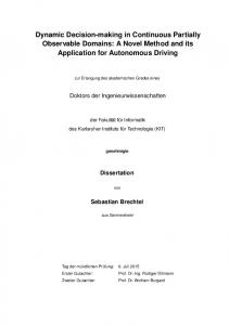
Fig. 1. Evolution of the discounted reward. There is a sudden change in the correct observation probability a time 0. Here, the equilibrium confidence is low (100).

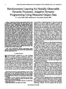
Fig. 2. Evolution of the discounted reward. There is a sudden change in the correct observation probability a time 0. Here, the equilibrium confidence is high (1000).

On Figure 1, we see the behavior of the algorithm when the equilibrium confidence is low (equal to 100): the agent quickly adapts to the new parameter value even if the variation is big. However the low confidence introduces some oscillations in the parameter values and therefore in the policy. In figure 2, we see what happens when the equilibrium confidence is high (equal to 1000): the agent takes more time to adapt to the new parameter value but the oscillations are less important. These results show that we can actually tune the confidence factors to make them adapted either to almost constant parameters or to quickly changing parameters. Note that on these experiments we need a number of queries which is between 300 and 500. Actually, the non-query learning introduced in this paper reduces the number of queries necessary in MEDUSA by a factor of 3.

6

Related Work

Chrisman (1992) was among the first to propose a method for acquiring a POMDP model from data. Shatkay & Kaelbling (1997) used a version of the Baum-Welch algorithm to learn POMDP models for robot navigation. Bayesian exploration was proposed by Dearden et al. (1999) to learn the parameters of an MDP. Their idea was to reason about model uncertainty using Dirichlet distributions over uncertain model parameters. The initial Dirichlet parameters can capture the rough model, and they can also be easily updated to reflect experience. The algorithm we present in Section 3 can be viewed as an extension of this work to the POMDP framework, though it is different in many respects, including how we trade-off exploration vs exploitation, and how we take nonstationarity into account. Recent work by Anderson and Moore (2005) examines the question of active learning in HMMs. In particular, their framework for model learning addresses a very similar problem (albeit without the complication of actions). The solution they propose selects queries to minimize error loss (i.e., loss of reward). However, their work is not directly applicable since they are concerned with picking the best query for a large set of possible queries. In our framework, there is only one query to consider, which reveals the current state. Furthermore, even if we wanted to consider a larger set of queries, their work would be difficult to apply since each query choice requires solving many POMDPs (where many means quadratic in the number of possible queries.) Finally, we point out that our work bears resemblance to some of the recent approaches for handling model-free POMDPs (McCallum, 1996; Brafman & Shani, 2005; Singh et al. 2004). Whereas these approaches are well suited to domains where there is no good state representation, our work does make strong assumptions about the existence of an underlying state. This assumption allows us to partly specify a model whenever possible, thereby making the learning problem much more tractable (e.g., orders of magnitude fewer examples). The other key assumption we make, which is not used in model-free approaches, regards the existence of an oracle (or human) for correctly identifying the state following each query. This is a strong assumption; however, in the empirical results we provide examples of why and how this can be at least partly relaxed. For instance, we showed that noisy query responses are sufficient, and that hyper-parameters can be updated even without queries.

7

Conclusion

We have discussed an active learning strategy for POMDPs which handles cases where we don’t know the full domain dynamics and cases where the model changes over time. Those were cases that no other work in the POMDP literature had handled. We have explained the MEDUSA+ algorithm and the improvements we made from MEDUSA. We have discussed the theoretical properties of MEDUSA+ and presented the conditions needed for its convergence. Furthermore, we have shown empirical results showing that MEDUSA+ can cope with non stationary POMDPs with a reasonable amount of experimentation.

References Anderson, B. and Moore, A. “Active Learning in HMMs”. In submission. 2005. Brafman, R. I. and Shani, G. “Resolving perceptual asliasing with noisy sensors”. Neural Information Processing Systems. 2005. Chrisman, L. “Reinforcement learning with perceptual aliasing: The perceptual distinctions approach”. In Proceedings of the Tenth International Conference on Artificial Intelligence, pages 183–188. AAAI Press. 1992. Cohn, D. A., Ghahramani, Z. and Jordan, M. I. “Active Learning with Statistical Models”. Advances in Neural Information Processing Systems. Dearden, R.,Friedman, N.,Andre, N., ”Model Based Bayesian Exploration”, Proc. Fifteenth Conf. on Uncertainty in Artificial Intelligence (UAI), 1999. Jaulmes, R.,Pineau, J.,Precup, D., ”Active Learning in Partially Observable Markov Decision Processes”, ECML, 2005. Kaelbling, L., Littman, M. and Cassandra, A. ”Planning and Acting in Partially Observable Stochastic Domains” Artificial Intelligence. vol.101. 1998. Littman, M., Cassandra, A., and Kaelbling,L. ”Learning policies for partially observable environments: Scaling up”, Brown University, 1995. McCallum, A. K. Reinforcement Learning with Selective Perception and Hidden State. Ph.D. Thesis. University of Rochester. 1996. Pineau, J., Gordon, G. and Thrun, S. “Point-based value iteration: An anytime algorithm for POMDPs”. IJCAI. 2003. Poupart, P. and Boutilier, C. “VDCBPI: an Approximate Scalable Algorithm for Large Scale POMDPs”. NIPS 2005. Shatkay, H., and Kaelbling, L. “Learning topological maps with weak local odometric information”. Proceedings of the Fifteenth International Joint Conference on Artificial Intelligence (pp. 920–927). Morgan Kaufmann. 1997. Singh, S., Littman, M., Jong, N. K., Pardoe, D., and Stone, P. “Learning Predictive State Representations”. Machine Learning: Proceedings of the 2003 International Conference (ICML). 2003. Spaan, M. T. J. Spaan, and Vlassis, N. “Perseus: randomized point-based value iteration for POMDPs”. Journal of Artificial Intelligence Research. 2005. To appear.