Sep 17, 2017 - Carnegie Mellon University. Pittsburgh, PA 15213 ... In our case, we consider the late 2000s financial crisis, which fundamentally altered.
arXiv:1709.05602v1 [stat.ML] 17 Sep 2017
Learning Mixtures of Multi-Output Regression Models by Correlation Clustering for Multi-View Data
Eric Lei Machine Learning Department Carnegie Mellon University Pittsburgh, PA 15213
Kyle Miller Auton Lab Carnegie Mellon University Pittsburgh, PA 15213
Abstract In many datasets, different parts of the data may have their own patterns of correlation, a structure that can be modeled as a mixture of local linear correlation models. The task of finding these mixtures is known as correlation clustering. In this work, we propose a linear correlation clustering method for datasets whose features are pre-divided into two views. The method, called Canonical Least Squares (CLS) clustering, is inspired by multi-output regression and Canonical Correlation Analysis. CLS clusters can be interpreted as variations in the regression relationship between the two views. The method is useful for data mining and data interpretation. Its utility is demonstrated on a synthetic dataset and stock market dataset.
1
Artur Dubrawski Auton Lab Carnegie Mellon University Pittsburgh, PA 15213
personality disorders (Sherry and Henson, 2005). If the views are considered input and output, data of this form can be a natural candidate for multi-output regression. We propose a novel technique inspired by multi-output regression called Canonical Least Squares (CLS) and apply it to clustering; CLS clusters can be interpreted as variations in the regression relationship between input and output views. The method is demonstrated on a synthetic dataset and stock market dataset.
INTRODUCTION
A common problem in data analysis is to investigate correlation structure. In many datasets, different parts of the data may have their own patterns of correlation. In general, clustering data based on local correlations is known as correlation clustering (Klami and Kaski, 2008; Zimek, 2009) (not to be confused with a machine learning graph problem of the same name). Additionally, there may be global nonlinear correlation structure in data. Both issues may be solved by mixing local linear correlation models and identifying them using a clustering method. In this work, we develop a linear correlation clustering method for datasets whose features are pre-divided into two views. These views can be arbitrary but usually correspond to two distinct facets of the data. This kind of duality occurs frequently in the real world: important examples include genes and diseases (Seoane et al., 2014), visuals and text (Rasiwasia et al., 2010), and emotions and
Figure 1: Histogram of pre- and post-crisis returns of Alexion Pharmaceuticals, a pharmaceutical company. We now explore a motivating example involving the stock market. One way to have two views of a time series such as stock returns is to consider temporal windows before and after some event. In our case, we consider the late 2000s financial crisis, which fundamentally altered some facets of the US economy. We hypothesize that the behavior of some stocks changed as a result of the crisis. For instance, Fig. 1 illustrates how the distribution of returns of one company differed before and after the crisis. The distribution became narrower and more symmetric and increased in mean. Granted, there are many factors
that can affect stock returns, but by considering hundreds of stocks we aim to isolate the systematic effect of the crisis. Our method lets us find clusters of stocks that exhibited similar changes and examine the nature of the changes. Another tool for analyzing data in two views is Canonical Correlation Analysis (CCA), a well-known statistical technique that discovers correlation structure between a pair of sets of random variables (Hotelling, 1936; Hardoon et al., 2004). CCA is the basis for a clustering method by Fern and Friedl (2005), and our clustering method uses CLS as its basis in an equivalent way. However, deep similarities to CCA notwithstanding, CLS clustering finds fundamentally different relationships. It also enjoys some practical advantages over CCA clustering. The paper is organized as follows: §2 summarizes related work; §3 gives necessary background on CCA; §4 derives the CLS clustering method; §5 describes experimental results; §6 discusses properties and uses of the method; and §7 concludes the paper.
2
RELATED WORK
Cluster-wise linear regression. Sp¨ath (1982) introduces a method for clustering the observations in a singleoutput regression dataset. Like k-means, this method is greedy and iterative and alternates between two steps. Given cluster labels, it fits a linear regression to each cluster. Given regression coefficients, it assigns each observation to the cluster whose regression residual is the smallest for that observation. It is simple to show that this method is a special case of CLS clustering in which the regression inputs are one set of variables and the regression output by itself is the other set—i.e., one view is univariate. Dependency seeking clustering. An interesting approach to correlation clustering is explored by Klami and Kaski (2008) and Rey and Roth (2012). Klami and Kaski (2008) establish a probabilistic generative modeling framework to allow Bayesian inference. They do so by proposing a model of probabilistic families for finding dependency and give a general clustering algorithm for this family. CCA is shown to be a special case. A key assumption is that a linearly transformed Gaussian latent variable produces the variation in the data. However, there may be severe model mismatch when this assumption was violated. To remedy this behavior, Rey and Roth (2012) deploy a copula mixture model to the framework, enabling them to model mixtures of CCA, similar to the clustering setup in this work. A Bayesian clustering algorithm is proposed and shown to perform well on synthetic and real datasets.
Multi-view clustering. There has been substantial past work on multi-view clustering. Multi-view versions of k-means and Expectation Maximization were considered by Bickel and Scheffer (2004) and found to outperform the single-view counterparts. A method by Chaudhuri et al. (2009) uses CCA to find the subspace spanned by the means of mixture components. The data are projected down to this subspace and clustered. In Kumar et al. (2011), a multi-view spectral clustering framework is proposed. This framework employs co-regularization to enforce agreement between clusterings in different views. Another line of work by Nie et al. (2011) and Wang et al. (2013) approaches clustering as a regression-like problem of fitting the data to cluster membership probabilities. The work of Wang et al. (2013) applies structured sparsity to weight features in different views by their importance. In addition, a method was proposed by Liu et al. (2013) that uses nonnegative matrix factorization. This method searches for matrix factorizations that give compatible clusters across the views. Single-view correlation clustering. Zimek (2009) considers the problem of clustering data based on patterns of correlation when the variables are not partitioned into two groups. At a high level, the paper’s definition of correlation clustering is similar to the definition in the CLS or CCA context: the task of separating observations into clusters that have distinct correlation structure. Unlike CLS or CCA, however, this work assumes a single view; the correlation refers to correlation between all the variables, not just between two sets. The paper presents a diverse body of algorithms for this task. Related to CLS clustering is a class of methods based on on Principal Components Analysis (PCA) (Zimek, 2009). A key intuition is that the principal components corresponding to lower eigenvalues resemble clusters because they have less variance. They then partition observations into clusters whose lower principal components are close together. These methods resemble CLS clustering in the way they leverage eigenvectors of lower variance.
3
BACKGROUND
In this section we describe CCA and CCA clustering. These methods serve as a useful starting point to understand CLS clustering. 3.1
CANONICAL CORRELATION ANALYSIS
CCA is a method for understanding cross-covariance between two sets of variables. Informally, it finds common signals between the sets. By performing CCA, one can understand how much variance in the sets can be explained by common factors. For example, if one set is
genes and the other is diseases, then CCA might connect combinations of genes with certain diseases, potentially corresponding to physiological traits. Formally, it finds maximally correlated linear combinations of each set. Let X ∈ Rd1 and Y ∈ Rd2 be random vectors. Without loss of generality, assume E[X] = E[Y ] = 0. Then CCA solves the problem max
u∈Rd1 ,v∈Rd2
Corr(X T u, Y T v).
(1)
Define ΣXY = Cov(X, Y ), ΣXX = Cov(X), and ΣY Y = Cov(Y ). The solution of (1) is wellunderstood (Hardoon et al., 2004): u is the leading eigenvector of −1 T A = Σ−1 XX ΣXY ΣY Y ΣXY and v the leading eigenvector of −1 T B = Σ−1 Y Y ΣXY ΣXX ΣXY .
Subsequent linear combinations can be found under the constraint that the previous components X T u and Y T v, known as canonical variables, are uncorrelated with the new canonical variables. Formally, let ui , vi , i = 1, . . . , m − 1, be the first m − 1 solutions. Then um and vm solve max
u∈Rd1 ,v∈Rd2
subject to
Corr(X T u, Y T v) Cov(Xu, Xui ) = Cov(Y v, Y vi ) = 0, i = 1, . . . , m − 1.
(2) For m ≤ min(d1 , d2 , rank(ΣXY )), the solutions to (2) are known to be the m-th leading eigenvectors of A and B. A standard reformulation (Hardoon et al., 2004) of (1) is max
u∈Rd1 ,v∈Rd2
The paper introduces an algorithm with a similar structure to k-means. Let X ∈ Rn×d1 and Y ∈ Rn×d2 be the data matrices corresponding to x and y. Let X (i) and Y (i) denote X and Y only with rows corresponding to samples assigned to cluster i. CCA clustering iterates two steps until convergence. The CCA step assumes cluster labels and runs CCA on each cluster, finding a linear regression between each pair of canonical variables. The labeling step assumes coefficients from CCA and linear regression and assigns each data point to the cluster that leads to the lowest weighted sum of squared residuals. Initialization can be arbitrary. • CCA step. Given cluster labels, for each cluster i = 1, . . . , k: run CCA on X (i) and Y (i) to find {uij } and {vij }, j = 1, . . . , m, and fit univariate linear regressions Y (i)T vij = αij + βij X (i)T uij . • Labeling step. Given CCA and regression coefficients {uij , vij , αij , βij }, for each observation (x` , y` ), ` = 1, . . . , n: assign it to
uT ΣXY v (3)
subject to uT ΣXX u = v T ΣY Y v = 1. The objective of (3) can also be expressed with the same constraints as � � (4) min E kXu − Y vk22 u∈Rd1 ,v∈Rd2
which resembles a least-squares problem. 3.2
varies between different subsets of samples or the global correlation structure is nonlinear, then CCA may be suboptimal. Instead, they consider a mixture of local CCA models to capture varying correlations and approximate global nonlinear correlations. Formally, given a dataset described by two sets of variables x and y, a hyperparameter for the number k of clusters, and a hyperparameter for the number m of canonical variables to use, the goal of CCA clustering is to partition the data into k clusters such that for instances in the same cluster, the features in x and y are correlated in the same way. Ideally, the correlation patterns differ between clusters, but this idea is not enforced. The paper also observes that if CCA finds strong correlations in a cluster, then the canonical variables can predict each other by linear regression.
CCA CLUSTERING
Fern and Friedl (2005) consider datasets split between two views and identify CCA as a useful tool to understand the correlations between them. However, they observe that CCA only detects linear correlations that are valid throughout the entire dataset. If the correlation structure
argmini
m X rij T 2 (y` vij − αij − βij xT ` uij ) r i1 j=1
where rij = Corr(X (i)T uij , Y (i)T vij ). CCA clustering is demonstrated to perform well on synthetic and earth science datasets. Nevertheless, there are a few considerations regarding CCA clustering. For one, it has no objective function. Although the paper gives its objective function as weighted prediction error, this function is only being optimized in the labeling step. Meanwhile, the CCA step maximizes correlation, which can increase the prediction error. Indeed, there appear to be two objectives, prediction error and correlation, which are related but not quite equivalent. It is unclear whether different solutions to CCA
maximum correlation but of least squared error. 0.75
4.1
FIRST COMPONENTS
0.7
For now, consider only using the first pair of components (m = 1). We start by examining the effect of the labeling step from CCA clustering on the CCA objective. Recall the formulation of CCA in (4). We redefine X ∈ Rn×d1 and Y ∈ Rn×d2 as centered data matrices. Then (4) becomes min kXu − Y vk22
Objective value
0.65 0.6 0.55 0.5 0.45
u∈Rd1 ,v∈Rd2
0.4
(i)
0.35 0
5
10
15
20
25
30
Epoch
Figure 2: CCA clustering non-convergence. On some data CCA clustering alternates between a set of cluster assignments, shown here by the oscillating objective.
Let R(i) be a square matrix of length n with R`` = 1 if point ` is in cluster i and all other entries 0. Then the CCA step for cluster i solves kR(i) (Xui − Y vi )k22
min
ui ∈Rd1 ,vi ∈Rd2
T (i) uT i X R Xui = 1
subject to
(5)
viT Y T R(i) Y vi = 1. X
4
The entire CCA step can be viewed as minimizing the sum of this objective for every cluster subject to all the constraints. Omitting constraints, this optimization problem is given by X min kR(i) (Xui − Y vi )k22 . (6)
Y
5
2 0
0
-2 -4 -5
0
5
ui ∈Rd1 ,vi ∈Rd2
i
-5 -5
0
5
Figure 3: Synthetic data from a mixture of two multivariate normal distributions on which CCA clustering fails to converge. Colors correspond to which normal distribution the point originated from. clustering should be compared by their prediction error or the strength of their correlations. In addition, there is no guarantee of convergence. We found that on certain distributions the method sometimes did not converge and experienced dramatic fluctuations in weighted prediction error, as in Fig. 2. These data were drawn from a mixture of two multivariate normals, shown in Fig. 3.
The labeling step chooses all R(i) to minimize linear regression error. We opt to instead choose R(i) to minimize (6), which means assigning each point to the cluster that minimizes the Euclidean distance between its components, skipping the linear regression step. Furthermore, in our method’s update step, which we name the CLS step, we, like in CCA, choose ui and vi to minimize (6). Where are our method differs, however, is the constraints: we only enforce viT vi = 1 and none of the constraints in (5), leading to the optimization problem X i
min
ui ∈Rd1 ,vi ∈Rd2
subject to
4
CANONICAL LEAST SQUARES CLUSTERING
In this section we develop a method for correlation clustering called Canonical Least Squares (CLS) clustering. First we introduce CLS, an analogue of CCA. Like CCA, CLS takes sets of variables X and Y and produces up to m ≤ min(d1 , d2 , rank(X T Y )) pairs of vectors (u, v) such that the components X T u and Y T v have some kind of relationship. Unlike CCA, this relationship is not of
kR(i) (Xui − Y vi )k22
viT vi
(7) = 1, i = 1, . . . , k.
This problem yields the first CLS components. A crucial difference from CCA is the lack of R(i) in the constraints. Thus the proposed labeling step minimizes (6) while respecting the constraints because they are independent of the cluster labels. As a result, both the CLS step and labeling step decrease the objective function. The other difference is the lack of ui in the constraints. These would serve no purpose in CLS; constraints on only vi suffice to eliminate the zero solution as the minimum. Additionally, when only vi is constrained, the problem generalizes
ordinary least squares, which does not constrain the coefficients of the independent variables. Next we present the solution for the first CLS component. We omit superscripts and subscripts involving i by considering only a single cluster. Furthermore, matrix R(i) can be omitted by considering only rows of X and Y that belong to cluster i. The problem is then given by min
u∈Rd1 ,v∈Rd2
kXu − Y vk22
subject to v T v = 1.
Let v be fixed. The problem becomes ordinary least squares in u, yielding u = (X T X)−1 X T Y v. Let H = I − X(X T X)−1 X T . After substituting for u, the problem in v is given by min kHY vk22
subject to v T v = 1.
v∈Rd2
This problem resembles PCA except with a minimum instead of maximum. The solution v is the eigenvector with the lowest eigenvalue of Y T H T HY = Y T HY . 4.2
MULTIPLE COMPONENTS
In CCA, subsequent canonical variables are uncorrelated with each other. After changing these constraints to be independent of the data, we are left with simple orthogonality constraints between vectors of coefficients. The generalization of (7) to m components is X i
min
U (i) ∈Rd1 ×m V (i) ∈Rd2 ×m
kR(i) (XU (i) − Y V (i) )k2F
subject to V
(8) (i)T
V
(i)
= I, i = 1, . . . , k.
This problem is non-convex in the constraints. It is difficult to solve because all components must be found simultaneously. We instead choose an easier suboptimal solution: let V (i) be the eigenvectors corresponding to the m lowest eigenvalues from the solution to (7), and compute U (i) accordingly. This solution corresponds to greedily solving for each component sequentially under orthogonality. It is an interesting tangent to juxtapose this procedure with Principal Components Analysis (PCA), which solves a similar problem max kZW k2F
W ∈Rd×d
subject to W T W = I
where Z ∈ Rn×d is a centered data matrix. In PCA, the greedy eigenvector solution is optimal because of the orthogonality constraints between full vectors of coefficients. In CLS, however, only the vectors vi must be orthogonal, rendering the greedy solution suboptimal.
Separately, in the special case that m = min{d1 , d2 }, then U or V is an orthogonal matrix, so CLS reduces to ordinary least squares on the columns of X or Y respectively. 4.3
CLUSTERING ALGORITHM
The CLS clustering algorithm takes matrices X and Y , a number k of clusters, and a number m of components. Let X (i) and Y (i) denote X and Y with rows subsampled to those in cluster i. To find cluster labels for each data point, we iterate the following steps until convergence: • CLS step Given cluster labels, for each cluster i = 1, . . . , k: run CLS on X (i) and Y (i) to find U (i) and V (i) . • Labeling step Given CLS coefficients U (i) and V i) , for each observation (x` , y` ), ` = 1, . . . , n: assign it to (i) 2 argmini ky`T V (i) − xT k2 . `U
The optimization problem solved by CLS clustering is given by (8). Also, it has a convergence guarantee when m = 1, i.e., when only the first pair of components is used. It is not unreasonable to use m = 1 because the first components are often the most meaningful. For m = 1, the optimization problem is given by (7). The CLS step optimizes over the ui ’s and vi ’s, while the labeling step optimizes over the R(i) ’s. Thus the objective is non-increasing at every step, so convergence is guaranteed. Even if m > 1, the greedy approximation of the CLS solution is usually non-increasing, which encourages convergence. Compared to CCA clustering, CLS clustering finds inherently different relationships by combining CCA and linear regression into a single step. Further analysis of the differences is given in the Discussion section. 4.4
PRACTICALITIES
Intercept. CCA clustering has an intercept term in its linear regression step. An intercept can be incorporated in CLS clustering as well by augmenting X with a column of 1’s. Data scale. CCA is affine invariant with respect to X and Y . However, CLS is sensitive because it uses Euclidean distance, similar to k-means. Therefore, we recommend normalizing the column variance in preprocessing.
Initialization. Like all greedy iterative algorithms similar to k-means, random initialization with many runs improves the chance of CLS clustering to achieve a robust solution.
5
RESULTS
5.1
SYNTHETIC DATASET
5.1.1
cide. Finding clusters of one kind would result in missing relationships of the other. First, spatial clusters were randomly sampled from two 2-dimensional normal distributions to form the X view. The spatial clusters in X were linearly transformed with noise to produce Y (Fig. 4). There were two separate linear transformations, each corresponding to a correlation cluster. The linear transformation to use was randomly selected for every point.
Description 5.1.2
X
Y
Actual clusters
4
5
2 0
0
-2 -4 -5
0
5
4
-5 -5
CLS clusters
R 2=0.65
2
R 2=0.93
R =0.93
0
0
-2 -4 -5
0
5
CCA clusters
4 2
-5 -5
0
5
5 R 2=0.69
R 2=0.69
R 2=0.88
R 2=0.88
0
0
In addition, spatial clusters were found by k-means with k = 4. Linear regressions were fitted from the X variables to the individual Y variables of each cluster. The maximum R2 over the Y variables is displayed in Fig. 4. This clustering approach was outperformed by CLS clustering. The k-means clusters could not identify the separate correlation structures because they were not distinguishable spatially. 5.2
STOCK MARKET DATASET
-2 -4 -5
0
5
4
k-means (k = 4)
5
Cluster assignments were found by CLS clustering and CCA clustering with k = 2 clusters and m = 1 components. Fig. 4 illustrates the cluster assignments as well as the R2 in each cluster on testing data sampled from the same distribution as the training data. The Pearson correlation between actual and predicted labels was 89% for CLS clusters and 57% for CCA clusters, a significant advantage for CLS clustering. CCA clustering underperformed largely because it grouped many points in the pink cluster when they were actually from the blue cluster.
5 R 2=0.65
2
0
Analysis
-5 -5
0
5
5
2 0
0
-2
R 2=0.43
R 2=0.43
R 2=0.11 R 2=0.52
R 2=0.11 R 2=0.52
2
-4 -5
R =0.38
0
5
-5 -5
R 2=0.38
0
5
CLS clustering is applied to stock market data with a focus on interpretation of clusters. Unlike most other multiview clustering methods (Chaudhuri et al., 2009; Kumar et al., 2011; Liu et al., 2013; Wang et al., 2013), this work is not especially suited for the plethora of multi-view datasets on which clustering techniques can be evaluated as unsupervised classification methods. Although CLS cluster variables are meaningful, they are usually not as straightforward as the target cluster variables in those datasets. 5.2.1
Figure 4: Comparison between cluster assignments of different methods on synthetic data. Also shown are the R2 values for the regression corresponding to each cluster. We performed a comparison of CLS clustering to other correlation clustering methods on synthetic data. This dataset was constructed to contain spatial clusters and correlation clusters where the two kinds did not coin-
Description
The financial crisis during 2007-2009 fundamentally altered some facets of the US economy. For example, it may have changed the distributions of returns of particular stocks. Stock returns, which typically have bellshaped distributions (Fama, 1965), could have shifted in mean, variance, or higher moments, as in Fig. 1. In this experiment we undertake a simplistic analysis of stock market data. These data are notoriously noisy and non-
stationary (Fama, 1965), so our analysis will avoid these nuances and focus on crude hypotheses. We also do not seek to employ macroeconomic reasoning to explain the underlying causes of the changes. We investigate whether stocks can be clustered based on how returns changed as the result of the crisis. Specifically, we employ temporal views of pre-crisis and post-crisis eras. We ask how the relationship between expected return, volatility of returns, and other features changed after the crisis and to what extent different changes reflect different clusters of stocks. By considering hundreds of stocks we aim to isolate the systematic effect of the crisis and reduce the effect of other factors. To select the data, we use the S&P 500, a stock market index composed of about 500 stocks of large US companies that is ubiquitous in finance literature. We examined data from the constituents it had on March 2nd , 2017. The date is important because the constituents regularly change. The monthly returns from July, 2004, to July, 2007, were designated as pre-crisis inputs, and those from August, 2009, to August, 2012, were designated as postcrisis outputs. The data were downloaded from Yahoo Finance, a free resource. The stocks with missing data were excluded, leaving 433 stocks. We performed two experiments corresponding to different feature sets. First, to allow simple illustrations, we extracted only two features in each view: the mean and standard deviation of (logarithmic) returns. These features are known as the expected return and volatility respectively. Second, to showcase the method with more informative features, we extracted six features per view: mean, standard deviation, skewness, and kurtosis of returns, along with beta and total trading volume. Beta is a measure of a stock’s sensitivity to movements of the aggregate S&P 500 index (Ross, 1976). The features were normalized to unit variance in both cases. 5.2.2
Two Feature Experiment
Pre-crisis
Post-crisis 0.1 1 2 3
0.05 0 -0.05
Expected return
0.1
Expected return
we set k = 3 clusters. We use m = 1 component. The cluster assignments found by CLS clustering are shown in Fig. 5. The plots of expected return versus volatility demonstrate the risk-reward trade-off of the stocks. In general, the risk (volatility) and reward (expected return) are positively correlated. However, different stocks can have a better or worse trade-off, indicated by lesser or greater slope from the origin respectively. Here, each cluster appears as a line, a linear relationship between expected return and volatility in the post-crisis view. This property is not coincidental; it is further explored in the Discussion section. Using this property, the clusters can be interpreted as follows: Clusters 1 (red) and 3 (blue) have an inverse relationship between risk and reward relative to the average trade-off, meaning their trade-offs deviate in either direction from the average. Cluster 1 contains overall lower expected returns and volatilities than Cluster 3. Meanwhile, Cluster 2 (green) exhibits an average trade-off between risk and reward.
0.05 1 2 3
0 -0.05
0.05
0.1
Volatility
0.15
0
0.1
0.2
Volatility
Figure 5: Cluster assignments of CLS in stock market data. In this experiment each view only had two features: expected return and volatility. For simplicity of analysis,
Figure 6: Individual CLS clusters in stock market data. Colors correspond to level sets of CLS component value. Although the clusters can be readily interpreted as above using only the post-crisis view, they are also characterized by subtle relationships to the pre-crisis view that are harder to visualize. In Fig. 6, each cluster is displayed separately. The colors correspond to level sets of CLS
component values, Xu and Y v. They provide a way to connect the same data point between views because almost every point is colored the same way in both views. In Cluster 1, they represent inverse relationships between expected return and volatility because of the downward slopes of each color line. The pre-crisis view reveals that any given line in the post-crisis view also corresponds to an inverse relationship between risk and reward in the pre-crisis view. In contrast, in Cluster 3, the same inverse relationship is present post-crisis, but each line corresponds to a proportional relationship pre-crisis. Described in basic terms, in Cluster 1 if one stock has lower volatility yet higher expected return than another post-crisis, then the same relationship is more likely to hold pre-crisis. However, in Cluster 3 if one stock has lower volatility yet higher expected return than another post-crisis, then the relationship is more likely to differ pre-crisis: one stock has higher volatility and expected return. The same reasoning can be applied to Cluster 2. If one stock has higher volatility and expected return than another, then the relationship is more likely to differ precrisis: one stock has lower volatility yet higher expected return.
and beta (in boldface), which are both measures of risk. Thus, the component can be interpreted as a regression on risk. On the pre-crisis side, it can be inferred from the coefficient signs that kurtosis and beta are positively correlated with post-crisis risk, while expected return, volatility, skewness, and volume are negatively correlated. These correlations are a distinguishing property of this cluster. Separately, this process motivates a need for a sparse version of CLS for easier interpretation of the coefficients. We leave this problem for future work. The number k = 5 of clusters and number m = 2 of components were selected by the elbow method (Ketchen, Jr. and Shook, 1996) applied to R2 averaged over the clusters and components (Fig. 7). Note that average R2 is lower with more components because the earlier components usually have higher R2 .
1 0.9 0.8
Six Feature Experiment
0.7
R2
5.2.3
In this experiment each view had six features: expected return, volatility, skewness of returns, kurtosis of returns, beta, and trading volume. We used k = 5 clusters and m = 2 components.
0.6 0.5 m m m m m
0.4 0.3
Table 1: Coefficients of Cluster 1 COMP. 1 COMP. 2 Feature Pre Post Pre Post Exp. Ret. -0.04 0.005 -0.04 -0.08 Volatility -0.03 0.04 -0.2 0.5 Skewness -0.04 -0.002 -0.07 0.03 Kurtosis -0.08 0.005 0.02 0.05 Beta -0.002 0.1 0.1 0.8 Volume 1.1 1 -0.1 -0.1
Since the data are difficult to visualize, we instead present the coefficients of a particular cluster as an example. The CLS coefficients for Cluster 1 are given in Table 1. These reveal relationships between pre- and post-crisis returns. In the first component, the coefficients on post-crisis are almost completely concentrated on volume (in boldface). Furthermore, this pattern was exhibited by two more clusters. It follows that some clusters can be characterized by the regression relationship between post-crisis volume and pre-crisis inputs. In the second component, the postcrisis coefficients are largely concentrated on volatility
= = = = =
1 2 3 4 5
0.2 1
2
3
4
5
6
7
8
9
10
k
Figure 7: Choosing k and m by the elbow method applied to average R2 of CLS clusters.
6
DISCUSSION
In the above experiments we demonstrated the utility of CLS clustering in finding correlation clusters. The method estimates regression relationships between two views of data using a generalization of linear regression and clusters points based on those relationships. CLS clustering can be useful when clusters heavily overlap in Euclidean space. We provided a synthetic example in which CLS clustering greatly outperformed the similar CCA clustering method as well as k-means. In addition, using a stock market dataset we illustrated how CLS clusters can offer subtle information about the way variables change after a major event. More generally, CLS clustering unsupervised method useful for data mining and interpretation. It
can be applied to any situation in which the relationship between two views varies. For instance, another application scenario might be a dataset containing a corpus of text as one view and audio from speakers reading the text as another view. It is conceivable that there is variation in the way certain speakers read certain texts—possibly in tone, tempo, and pitch—depending on the type of text. The nature of the correlation between audio and text could be investigated by our method. We finish with some remarks about practical and theoretical properties of CLS clustering.
potentially overlapping linear subspaces such as in Fig. 4 and 5. These patterns in Euclidean space offer an alternative, more concrete means of interpretation than the more abstract correlations between linear combinations. The reason for this behavior is that for a linear subspace orthogonal to a vector v of projection coefficients, points in Y in and around the subspace are clustered around zero in the projected space. Due to less variance they tend to be easier to predict from X and are consequently clustered together.
7 Robustness Over Many Runs. CLS clustering solutions on the same data may differ depending on initialization. Fortunately they can be compared through the objective function. In contrast, CCA clustering solutions are less straightforward to compare because the objective function is not meaningful. One would have to employ heuristics such as average R2 . Therefore, one can be more confident about the quality of CLS clustering after many runs than CCA clustering. Goodness of Fit. Minimizing the squared error in CLS is not equivalent to maximizing R2 between Xu and Y v, which is the objective of CCA. Instead, CLS can find components with weaker correlation but smaller residuals. This difference is not necessarily detrimental because smaller residuals could be a plausible characteristic for identifying clusters. In fact, even CCA clustering does not maximize R2 in every cluster. While the update step of CCA certainly does, the labeling step can lower it in some clusters. Spectral Interpretation. Recall that the solution v for the first component of CLS was given by the last eigenvector of Z ≡ Y T (I − X(X T X)−1 X T )Y . Let Σxx = X T X, Σxy = X T Y , and Σyy = Y T Y . Assuming the data are centered, these variables are covariance and cross-covariance matrices of X and Y . Then −1 Z = Σyy − ΣT xy Σxx Σxy is the Schur complement of the covariance matrix of the joint distribution of X and Y . If this joint distribution is multivariate normal, then Z is the conditional covariance of Y given X. Hence CLS can be interpreted as finding the direction of minimum variance in Y given X. When Y has less variance after controlling for its relationship with X, it is easier to find a better linear fit with X. CLS clustering is similar in this regard to correlation clustering methods by Zimek (2009), which also leverage eigenvectors of lower variance. Contiguousness of Clusters in Output View. The CLS clusters tend to be more contiguous in Euclidean space in the Y view. In particular, they tend to follow
CONCLUSION
We have proposed a mixed local linear correlation model for clustering data with nonlinear or local correlation structure called Canonical Least Squares (CLS) clustering. CLS combines CCA and linear regression into a single operation to extract linear relationships between two sets of variates, similar to multi-output regression. This method is useful for data mining and interpretation. CLS clustering is to some extent similar to the earlier method of CCA clustering (Fern and Friedl, 2005) but is different mathematically and in other ways. For example, it has a well-defined objective function and a convergence guarantee when using one component. Also, its robustness can be improved by using many random initializations. Empirical results demonstrate that CLS clustering can outperform CCA clustering and find interpretable relationships.
References Bickel, S. and Scheffer, T. (2004). Multi-view clustering. In IEEE International Conference on Data Mining, number December 2004, pages 19–26. Chaudhuri, K., Kakade, S., Livescu, K., and Sridharan, K. (2009). Multi-view clustering via canonical correlation analysis. In International Conference on Machine Learning, pages 1–8. Fama, E. F. (1965). The behavior of stock-market prices. The Journal of Business, 38(1):34–105. Fern, X. and Friedl, M. (2005). Correlation clustering for learning mixtures of canonical correlation models. In SIAM International Conference on Data Mining, pages 439–446. Hardoon, D. R., Szedmak, S., and Shawe-Taylor, J. (2004). Canonical correlation analysis: An overview with application to learning methods. Neural Computation, 16(12):2639–2664. Hotelling, H. (1936). Relations between two sets of variates. Biometrika, 28(3/4):321–377. Ketchen, Jr., D. and Shook, C. (1996). The application of cluster analysis in strategic management research: An analysis and critique. Strategic Management Journal, 17(6):441–458. Klami, A. and Kaski, S. (2008). Probabilistic approach to detecting dependencies between data sets. Neurocomputing, 72(1):39–46. Kumar, A., Rai, P., and Daum´e, H. (2011). Co-regularized Multi-view Spectral Clustering. Neural Information Processing Systems, pages 1413–1421. Liu, J., Wang, C., Gao, J., and Han, J. (2013). Multi-view clustering via joint nonnegative matrix factorization. In SIAM International Conference on Data Mining, pages 252–260. Nie, F., Zeng, Z., Tsang, I., Xu, D., and Zhang, C. (2011). Spectral embedded clustering: A framework for insample and out-of-sample spectral clustering. IEEE Transactions on Neural Networks, 22(11):1796–1808. Rasiwasia, N., Costa Pereira, J., Coviello, E., Doyle, G., Lanckriet, G. R., Levy, R., and Vasconcelos, N. (2010). A new approach to cross-modal multimedia retrieval. In ACM International Conference on Multimedia, pages 251–260. ACM. Rey, M. and Roth, V. (2012). Copula mixture model for dependency-seeking clustering. International Conference on Machine Learning. Ross, S. A. (1976). The arbitrage theory of capital asset pricing. Journal of Economic Theory, 13(3):341–360.
Seoane, J. A., Campbell, C., Day, I. N., Casas, J. P., and Gaunt, T. R. (2014). Canonical correlation analysis for gene-based pleiotropy discovery. PLoS Compututational Biology, 10(10):e1003876. Sherry, A. and Henson, R. K. (2005). Conducting and interpreting canonical correlation analysis in personality research: A user-friendly primer. Journal of Personality Assessment, 84(1):37–48. Sp¨ath, H. (1982). A fast algorithm for clusterwise linear regression. Computing, 29(2):175–181. Wang, H., Nie, F., and Huang, H. (2013). Multi-view clustering and feature learning via structured sparsity. In International Conference on Machine Learning, volume 28, pages 352–360. Zimek, A. (2009). Correlation clustering. ACM SIGKDD Explorations, 11(1):53–54.