The options framework (Precup, 2000; Sutton, Precup & Singh,. 1999) provides a natural way of incorporating such actions into reinforcement learning systems ...
Learning Options in Reinforcement Learning Martin Stolle1 and Doina Precup1 School of Computer Science, McGill University, Montreal, QC, H3A 2A7, Canada mstoll,dprecup � @cs.mcgill.ca, �� � WWW home page: http://www.cs.mcgill.ca/ mstoll, dprecup �
Abstract. Temporally extended actions (e.g., macro actions) have proven very useful in speeding up learning, ensuring robustness and building prior knowledge into AI systems. The options framework (Precup, 2000; Sutton, Precup & Singh, 1999) provides a natural way of incorporating such actions into reinforcement learning systems, but leaves open the issue of how good options might be identified. In this paper, we empirically explore a simple approach to creating options. The underlying assumption is that the agent will be asked to perform different goal-achievement tasks in an environment that is otherwise the same over time. Our approach is based on the intuition that “bottleneck” states, i.e. states that are frequently visited on system trajectories, could prove to be useful subgoals (e.g. McGovern & Barto, 2001; Iba, 1989). We present empirical studies of this approach in two gridworld navigation tasks. One of the environments we explored contains bottleneck states, and the algorithm indeed finds these states, as expected. The second environment is an empty gridworld with no obstacles. Although the environment does not contain bottleneck states, our approach still finds useful options, which essentially allow the agent to travel around the environment more quickly.
1 Introduction Temporally extended actions (e.g., macro actions) have proven very useful in speeding up learning and planning, ensuring robustness and building prior knowledge into AI systems (e.g., Fikes, Hart, and Nilsson, 1972; Newell and Simon, 1972; Sacerdoti, 1977; Korf, 1987; Laird et al., 1986; Minton, 1988; Iba, 1989). More recently, the topic has been explored in the context of Markov Decision Processes (MDPs) and reinforcement learning (RL) (e.g., Singh, 1992; Parr, 1998; Dietterich, 1998; Precup, 2000). The options framework (Precup, 2000; Sutton, Precup & Singh, 1999) provides a natural way of incorporating extended actions into reinforcement learning systems. An option is specified by a set of states in which the option can be initiated, an internal policy and a termination condition. If the initiation set and the termination condition are specified, traditional reinforcement learning methods can be used to learn the internal policy of the option. One interesting issue that is left open in the options framework is that of automatically finding initiation sets and termination conditions for options. In this paper, we empirically explore a simple approach to creating options. The underlying assumption
is that the agent will be asked to perform different goal-achievement tasks in an environment that is otherwise the same over time. Our approach is based on the intuition that “bottleneck” states, i.e., states that are frequently visited on system trajectories, could prove to be useful subgoals (e.g. McGovern & Barto, 2001; Iba, 1989). The agent is first allowed to explore the environment and gather statistics, based on which it chooses potential subgoals and initiation states for the options. In the second phase, the agent learns the internal policies of the options. Once these are learned, the agent can use the options to solve the goal-achievement tasks it is presented with. We present empirical studies of this approach in two gridworld navigation tasks. One of the environments we explored contains bottleneck states, and the algorithm indeed finds these states, as expected. The second environment is an empty gridworld with no obstacles. Although the environment does not contain bottleneck states, this approach still finds useful options, which essentially allow the agent to travel around the environment more quickly. The paper is organized as follows. In section 2 we introduce the basic reinforcement learning notation. Section 3 contains the definition of options and SMDP Q-learning, the main algorithm we use for learning how to choose among options. In section 4 we describe our algorithm for automatically creating options. Section 5 contains empirical results of this algorithm for two gridworld tasks, and a discussion of the behavior we observed.
2 Reinforcement Learning Reinforcement learning (RL) is a computational approach to automating goal-directed learning and decision making (Sutton & Barto, 1998). It encompasses a broad range of methods for determining optimal ways of behaving in complex, uncertain and stochastic environments. Most current RL research is based on the theoretical framework of Markov Decision Processes (MDPs) (Puterman, 1996). MDPs are a standard, very general formalism for studying stochastic, sequential decision problems. In this framework, the agent takes a sequence of primitive actions paced by a discrete, fixed time scale. On each time step t, the agent observes the state of its environment, st , contained in a finite discrete set � , and chooses an action, at , from a finite action set � (possibly dependent on st ). One time step later, the agent receives a reward rt � 1 and the environment transitions to a next state, st � 1 . For a given state s and action a, the expected value of the immediate reward is rsa and the transition to a new state s� has probability pass� , regardless of the path taken by the agent before state s. A way of behaving, or policy, is defined as probability distribution for picking actions in each state: π : � �� �� 0 � 1� . The goal of the agent is to find a policy that maximizes the total reward received over time. For any policy π and any state s ��� , the value of taking action a in state s under policy π, denoted Qπ � s � a � , is the expected discounted future reward starting in s, taking a, and henceforth following π: Qπ � s � a �
def �
�
Eπ rt �
1�
γrt �
2 ���������
�
�
st
�
s � at
�
a� �
The optimal action-value function is: def � Q! � s � a � max Qπ � s � a �"� π
In an MDP, there exists a unique optimal value function, Q ! � s � a � , and at least one optimal policy, π ! , corresponding to this value function: π ! � s � a �$# 0 iff a � argmaxa�&%(' Q ! � s � a� � . Many popular reinforcement learning algorithms aim to compute Q ! (and thus implicitly π ! ) based on the observed interaction between the agent and the environment. The most widely-used is propably Q-learning (Watkins, 1989), which allows learning Q ! directly from interaction with the environment. The agent updates its value function as follows: Q � st � at �*) Q � st � at � α � rt � 1 � γ max Q � st � 1 � a� ��+ Q � st � at �,� a� %('
Q-learning has been shown to converge in the limit, with probability 1, to the optimal value function Q ! , under standard stochastic approximation assumptions.
3 Options Options (Precup, 2000; Sutton, Precup & Singh, 1999) are a generalization of primitive actions to include temporally extended courses of action. Options consist of three components: a policy π : �� -�/. 0� 0 � 1� , a termination condition β : �1. 0� 0 � 1� , and an input set 2435� . An option 6 27� π � β # is available in state s if and only if s �82 . If the option is taken, then actions are selected according to π until the option terminates stochastically according to β. That is, in state st the next action at is selected according to the probability distribution π � st � � � . The environment then makes a transition to state st � 1 , where the option either terminates, with probability β � st � 1 � , or else continues, determining at � 1 according to π � st � 1 � � � , possibly terminating in st � 2 according to β � st � 2 � , and so on. When the option terminates, then the agent has the opportunity to select another option. Note that primitive actions can be viewed as a special case of options. Each action �/9 a corresponds to an option that is available whenever a is available ( 2 s : a �:� s ; ), � � that always lasts exactly one step (β s � 1 �=< s �>� ), and that selects a everywhere � (π � s � a �?< s �@2 ). Thus, we can consider the agent’s choice at each time to be entirely among options, some of which persist for a single time step, others which are temporally extended. It is natural to generalize the action-value function to an option-value function. We define Qµ � s � o � , the value of taking option o in state s �A2 under policy µ, as �
Qµ � s � o � =.E rt �
1�
γrt �
2�
γ2 rt �
E � oµ � s � t � � �
3 ������� �
�
(1)
�
where oµ denotes the policy that first follows o until it terminates and then initiates µ in the resulting state, and E � oµ � s � t � denotes the execution of oµ in state s starting at time t. Options are closely related to the actions in a special kind of decision problem known as a semi-Markov decision process, or SMDP (e.g., see Puterman, 1994). In fact,
any MDP with a fixed set of options is an SMDP. Accordingly, the theory of SMDPs provides an important basis for a theory of options. The problem of finding an optimal policy over a set of options B can be addressed by learning methods. Because the MDP augmented by the options is an SMDP, we can apply SMDP learning methods as developed by Bradtke and Duff (1995), Parr and Russell (1997), Mahadevan (1996), or McGovern, Sutton and Fagg (1997). When the execution of option o is started in state s, we next jump to the state s� in which o terminates. Based on this experience, an option-value function Q � s � o � is updated. For example, the SMDP version of one-step Q-learning (Bradtke and Duff, 1995), updates the value function after each option termination by Q � s � o �C)
Q � s � o � � α D r � γk max Q � s� � a ��+ Q � s � o �HGI� a %FE
(2)
where k denotes the number of time steps elapsing between s and s� , r denotes the cumulative discounted reward over this time, and it is implicit that the step-size parameter α may depend arbitrarily on the states, option, and time steps. The estimate Q � s � o � converges to the optimal value function over options, Q !E � s � o � for all s �J� and o �8B under conditions similar to those for conventional Q-learning (Parr, 1998).
4 Finding Options If an initiation set and a termination condition are specified, the internal policies of options can be learned using standard RL methods (e.g. Q-learning, like in Precup, 2000). But the key issue remains how to select good termination conditions and initiation sets. Intuitively, it is clear that different heuristics would work well for different kinds of environments. In this paper, we assume that the agent is confronted with goal-achievement tasks, which take place in a fixed environment. This setup is quite natural when thinking about human activities. For instance, every day we might be cooking a different breakfast, but the kitchen layout is the same from day to day. We allow the agent to explore the environment ahead of time, in order to learn options. The option finding process is based on posing a series of random tasks in this environment and letting the agent solve them. During this time, the agent gathers statistics regarding the frequency of occurence of different states. Our algorithm is based on the intuition that, if states occur frequently on trajectories that represent solutions to random tasks, then these states may be important. Hence, we ill learn options that use these states as targets. The options finding algorithm is described in detail below. 1. Select at random a number of start states S and target states T that will be used to generate random tasks for the agent. 2. For each pair K S � T L (a) Perform Ntrain episodes of Q-learning, to learn a policy for going from S to T (b) Perform Nt est episodes using the greedy policy learned. For all states s, count the total number of times n � s � that each state is visited during these trajectories. 3. Repeat until the desired number of options is reached:
�
(a) Pick the state with the most visitations, Tmax arg maxs n � s � , as the target state for the option (b) Compute n � s � Tmax � , the number of times each state s occurs on paths that go through Tmax � (c) Compute n¯ � Tmax � avgs n � s � Tmax � . (d) Select all the states s for which n � s � Tmax �M# n¯ � Tmax � to be part of the initiation set 2 for the option. (e) Complete the initiation set by interpolating between the selected states. The interpolation process is domain-specific 4. For each option, learn its internal policy; this is achieved by giving a high reward for entering Tmax , and no rewards otherwise. The agent performs Q-learning, by performing episodes which start at random states in 2 and end when Tmax is reached, or when the agent exists 2 . Once the options are found, we use SMDP Q-learning, as described in the previous section, in order to learn a policy over options. Note that our approach is quite similar in spirit to that of McGovern and Barto (1998; 2001). But they are using data mining techniques (in particular diverse density) to learn from “good” and “bad” trajectories. We treat all trajectories in the same way. Our approach is probably the simplest implementation for the “bottleneck” state idea.
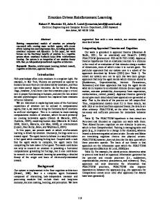
5 Experimental Results We experimented with this algorithm for finding options in two simple gridworld navigation tasks. The first one is the rooms environment depicted in Figure 1 (left panel). The state is the current cell position. There are four deterministic primitive actions which move the agent up, down, left and right. If the agent attempts to move into a wall, it stays in the same position, and no penalty is incurred. The discount factor is � γ 0 � 9 and there are no intermediate rewards anywhere. The agent can only obtain a reward upon entering a designated goal state. We assume that the goal state may move from one location to another over time. The hallway states are obvious bottleneck states in this environment, since trajectories passing from one room to another have to pass through the hallways. Hence, one would expected the option finding algortihm to work well in this context, finding options for going to the hallways.
ROOM
HALLWAYS
primitive actions up left
NO
Q
Q
Q Q Q Q Q Q
P Q
right down
Fig. 1. Rooms environment, and example option
We performed 30 independent runs of the algorithm. During each run, the option finding algorithm was used to find 8 options. During the option finding stage, 25% of the � states were used as potential start and goal states for random tasks. We used Ntrain 200 episodes to learn Q-values for each pair of start and goal states. After learning, we � used Ntest 10 episodes to generate the state visitation counts. The initiation sets were constructed by creating a rectangular box around the selected initiation states for each option. This approach is specific for gridworld navigation, and would not be expected to work well in other domains. After the initiation sets and the targets of the options were selected, the internal policy of each option was found using Q-learning for 100 trials. One example of an option found by the algorithm is depicted in Figure 1 (right panel). The target state for the option is close to one of the hallways, but not exactly in the hallway. This behavior was consistent across all runs, and is due to the fact that the states near the hallways are traversed both by trajectories going between rooms and by trajectories inside a room. This behavior is also consistent with earlier findings of McGovern (1998). The figure also shows that the option policy has been learned for most initiation states, although some states have a suboptimal policy, while others have still not been visited (and hence have a random policy).
550
5000 Primitives and Options Primitives only
500
Primitives only Primitives and Options 4500
450
4000
400 3500
Episode length
Episode length
350 300 250
3000
2500
2000
200 1500 150 1000
100
500
50 0
0
100
200
300 Episodes
400
500
600
0
0
100
200
300 Episodes
400
500
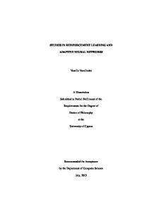
Fig. 2. Results for rooms environment
Once the options were learned, we compared the performance of a learning agent using primitive actions only to the performance of an agent using both primitive actions � and options. Both agents used a learning rate α 0 � 1 and ε-greedy policy for generating � behavior, with ε 0 � 1.We picked four different goal locations. The agents were trained for 150 episodes using a fixed goal location. Every episode consists of starting at a randomly chosen location and performing navigation actions until the goal is reached. After each 20 training episodes, we performed 5 test episodes, starting at random states and using the greedy policy to choose actions. After 150 episodes, the goal was moved, but the Q-values of each agent were retained, and the whole process was repeated. The results for the rooms environment are depicted in Figure 2. The left graph shows performance during training, while the right graph shows the performance of the greedy
600
policy learned. As expected, using temporally extended options provides and advantage over using primitive actions only, although the number of actions to learn about has increased from 4 to 12. Preliminary results indicate that this advantage would be even larger if we would use a more efficient learning method, such as intra-option learning. The second envioronment we experimented with was an empty 11 11 gridworld, with no obstacles. In this environemnt, there are no bottleneck states. Hence, it is not obvious that the option-finding heuristic would work well. Our inital expectation was that the use of the options found would actually slow down learning.
550
1200 Primitives and Options Primitives only
500
Primitives only Primitives and Options
1000
450 400
800 Episode length
Episode length
350 300 250
600
200 400 150 100
200
50 0
0
100
200
300 Episodes
400
500
600
0
0
100
200
300 Episodes
400
500
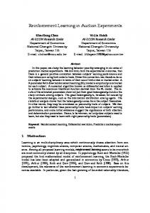
Fig. 3. Results for the empty gridworld environment. The left panel shows the performance during training, and the right panel shows the performance of the greedy policy learned.
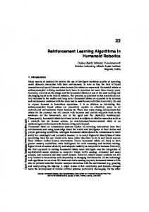
We applied our algorithm to this environment in the same manner described above. The results are depicted in Figure 3. During training, it is clear that the use of temporally extended options is helpful. The result is not so clear for the greedy policy, though. In order to understand better the behavior of the algorithm, we looked at the options that were found in this environment. On every run, the algorithm first found one (or a couple) of options leading to one of the central states in the environment. Once the state visitation counts were decreased by eliminating the trajectories that went through the center states, the peak counts were spread over states in different areas of the grid. Hence, on virtually every run, the algorithm found some options for navigating to different parts of the grid. Of course, such options are useful in the case in which the goal state moves around the environment. One example of the goal states found is depicted in Figure 4. The goals are numbered in the order in which they were selected.
6 Future work There are a lot of directions to be explored in option creation. We are currently investigating the use of more sophisticated learning and execution methods, such as intraoption learnign and early termination, with our option finding heuristics. Also, note
600
6 2 3 7
1
5
8 4
Fig. 4. Option target states found during one run in the empty gridworld.
that our algorithm is currently using the assumption that a tabular representation of the value functions is possible. We are looking into way of lifting this assumption
References Dietterich, T. G. (1998). Hierarchical reinforcement learning with the MAXQ value function decomposition. Seventeenth International Conference on Machine Learning (ICML’98). Fikes, Hart and Nilsson (1972). Learning and Executing Generalized Robot Plans. Artificial Intelligence, vol. 3, pp. 251–288 Iba, G. A. (1989). A heuristic approach to the discovery of macro-operators. Machine Learning, 3:285-317 Korf, R. E. (1985). Macro-operators: A weak method for learning. Artificial Intelligence, 26:35-77 Laird, J. E., Rosenbloom, P.S., and Newell, A. (1986). Chunking in Soar: The anatomy of a general learning mechanism. Machine Learning, 1:11-46 McGovern, A., and Sutton, R.S. (1998). Macro-actions in reinforcement learning: An empirical analysis. Technical Report 98-70, University of Massachusetts, Department of Computer Science. McGovern, A., and Barto, A.G. (2001). Automatic Discovery of Subgoals in Reinforcement Learning Using Diverse Densiti. Proceedings of the Eighteenth Intermational Conference on Machine Learning, ICML’01, pp. 361-368. Parr, R., and Russell, S. (1997). Reinforcement Learning with Hierarchies of Machines. NIPS 97. Sutton, R.S., Precup, D., Singh, S. (1999). Between MDPs and semi-MDPs: A Framework for Temporal Abstraction in Reinforcement Learning. Artificial Intelligence 112:181-211