Learning Predictive State Representations Using Non-Blind Policies

Learning Predictive State Representations Using Non-Blind Policies

Michael Bowling BOWLING @ CS . UALBERTA . CA Peter McCracken PETERM @ CS . UALBERTA . CA Department of Computing Science, University of Alberta, Edmonton, Alberta, T6G 2E8 Canada Michael James MICHAEL . R . JAMES @ GMAIL . COM AI and Robotics Group, Technical Research Dept., Toyota Technical Center, Ann Arbor, Michigan, USA James Neufeld NEUFELD @ CS . UALBERTA . CA Department of Computing Science, University of Alberta, Edmonton, Alberta, T6G 2E8 Canada Dana Wilkinson School of Computer Science, University of Waterloo, Waterloo, Ontario, Canada

Abstract Predictive state representations (PSRs) are powerful models of non-Markovian decision processes that differ from traditional models (e.g., HMMs, POMDPs) by representing state using only observable quantities. Because of this, PSRs can be learned solely using data from interaction with the process. The majority of existing techniques, though, explicitly or implicitly require that this data be gathered using a blind policy, where actions are selected independently of preceding observations. This is a severe limitation for practical learning of PSRs. We present two methods for fixing this limitation in most of the existing PSR algorithms: one when the policy is known and one when it is not. We then present an efficient optimization for computing good exploration policies to be used when learning a PSR. The exploration policies, which are not blind, significantly lower the amount of data needed to build an accurate model, thus demonstrating the importance of non-blind policies.

1. Introduction Predictive state representations (PSRs) are a method of representing the state of a controlled, discrete-time, stochastic dynamical system by maintaining predictions about the effect of future actions on observations (Littman et al., 2002). Appearing in Proceedings of the 23 rd International Conference on Machine Learning, Pittsburgh, PA, 2006. Copyright 2006 by the author(s)/owner(s).

D 3 WILKIN @ UWATERLOO . CA

PSRs have several advantages over other methods of state representation, such as POMDPs and k-Markov models. It has been shown that PSRs are able to compactly model any system representable by a POMDP (Singh et al., 2004) or k-Markov model (Littman et al., 2002). Also, unlike POMDPs which use a postulated set of underlying, nominal states, PSRs are completely specified using observable quantities like actions and observations. This allows them to be learned solely using data from interaction with the system. There have been numerous algorithms proposed for building PSR models from data (Singh et al., 2003; James & Singh, 2004; Rosencrantz et al., 2004; Wolfe et al., 2005; Wiewiora, 2005; McCracken & Bowling, 2006). Many of these algorithms specify a particular policy to be used when gathering their data. Those that do not are usually evaluated using the uniform-random policy. In either case the policy is blind, ignoring preceding observations when selecting actions. To date all of the policies used in PSR empirical evaluation have been blind. Generally speaking, though, non-blind policies are the norm not the special case. Selecting actions based on past observations is key for any policy seeking to maximize reward or achieve some goal. Even a smart exploration strategy will make decisions based on past observations. The ability to build accurate models from data gathered while purposefully exploring or acting to maximize reward is fundamental. In this paper we examine the construction of PSR models from data gathered while following non-blind policies. In particular, we conclude that most existing algorithms fail to build a correct model when data is gathered with such a policy. We start with a brief introducion to PSRs in Section 2. In Section 3 we prove that the majority of existing

Learning Predictive State Representations Using Non-Blind Policies

β

L

α

Pr(0) = 0.9 Pr(1) = 0.1

R Pr(0) = 0.1 Pr(1) = 0.9

β

α

Table 1. Two policies for the system in Figure 1. Policy 1 is dependent on the previous observation, and Policy 2 is blind. ‘∗0’ and ‘∗1’ represent any history that ends in observation 0 and 1, respectively.

Figure 1. A dynamical system with two nominal states, action set A = {α, β}, and observation set O = {0, 1}. Action α switches state, and action β preserves state. The initial state of the system is state L.

algorithms are only correct if data is gathered with a blind policy. We then show in Section 4 how existing algorithms can be fixed to handle data from any policy, known or unknown. In Section 5 we present a novel method for finding smart exploration policies which are not blind. We then show results in Section 6 when learning with these policies, demonstrating the correctness and usefulness of our remedy.

2. Background A controlled, discrete-time, finite dynamical system generates observations from a set O in response to actions from a set A. The probability of a generated observation, though, can depend on the complete interaction to date. An example dynamical system is shown in Figure 1. This system has two nominal states {L, R}, actions A = {α, β} and observations O = {0, 1}. An interaction with a dynamical system can be represented as a stream of action-observation pairs, of the form a1 o1 a2 o2 . . ., that begins at time step zero. In such a sequence, the first action taken is a1 , after which the observation o1 is observed, followed by action a2 and observation o2 , etc., until the end of the interaction. A sequence of action-observation pairs that has already occurred is referred to as a history. The special history, φ, is the zero-length history where no actions have been taken. At its essence a system is a probability distribution over observations, conditioned on the history and next action. For example, the system in Figure 1 can be described as,  0.9 if s(ha) = 0 mod 2 Pr(0|ha) = , 0.1 if s(ha) = 1 mod 2 where s(h) is the number of α, or switching, actions in h. POMDPs (or HMMs in the uncontrolled case), k-Markov models, and PSRs are simply compact models of this infinite set of probability distributions. A policy is a probability distribution over actions, conditioned on history. Example policies are shown in Table 1. A policy can rely on previous observations, like Policy 1 in Table 1, or it can be blind to previous observations, like Policy 2. A policy is said to be blind if each policy action is conditionally independent of previous observations,

h φ ∗0 ∗1

Policy 1 Pr(α|h) Pr(β|h) 0.5 0.5 0.9 0.1 0.1 0.9

Policy 2 Pr(α|h) Pr(β|h) 0.5 0.5 0.5 0.5 0.5 0.5

given previous actions. It should be noted that blind policy actions are not necessarily independent of previous observations. If action a2 depends on action a1 , and observation o1 depends on a1 , then a2 and o1 may not be (statistically) independent. A policy and a system together define a complete probability distribution on histories. The following convenient notation summarizes the contributions of the policy and the system for a particular history, π(a1 o1 . . . an on ) ≡ p(a1 o1 . . . an on ) ≡

n Y i=1 n Y

Pr(ai |a1 o1 . . . oi−1 ) Pr(oi |a1 o1 . . . ai ).

i=1

Using this notation the probability of any history is Pr(h) = π(h)p(h). We will also use the notation, n

π(t|h) ≡

π(ht) Y = Pr(ai |ha1 o1 . . . oi−1 ) π(h) i=1

p(t|h) ≡

p(ht) Y = Pr(oi |ha1 o1 . . . ai ), p(h) i=1

n

where t = a1 o1 . . . an on . 2.1. Predictive State Representations A test is a sequence of action-observation pairs that may occur in the future. A test t = a1 o1 . . . an on succeeds if the observation sequence of the test, o1 , . . . , on , is observed when the action sequence, a1 , . . . , an , is taken. The null test, ε, is the zero length test that, by definition, always succeeds. The prediction for a test t from a particular history h is the probability that the test will succeed, which we define to be p(t|h).1 1

We use a mathematical definition of prediction that differs from the literature. Traditionally p(t|h) is written as Pr(o1 . . . on |ha1 . . . an ), where the actions of the test appear to be random variables in the conditional probability. But they are not. They are best thought of as parameters of the joint distribution. In this work we are interested in actions as random variables and so use the more complicated but unambiguous definition.

Learning Predictive State Representations Using Non-Blind Policies

Suppose there exists a finite set of tests, Q, such that the prediction for any test can be written as a linear combination of predictions of tests in Q. Then we can model the system compactly as a predictive state representation. Formally, let p(Q|h) be the row vector of predictions for the tests in Q at history h. So, for all tests t, there exists a column vector mt such that ∀h p(t|h) = p(Q|h)mt . We will call such a Q, a set of core tests for the system.

are collected through interaction with the system and then used to choose core tests and approximate initial prediction and weight vectors. Many approaches proceed in an iterative fashion: alternating between gathering data for Monte Carlo estimates and using the estimates to find core tests and update vectors. This paper focuses on this broad class of algorithms, mainly concentrating on how prediction estimates are made from data.

A PSR summarizes histories (i.e., represents state) using predictions of the core tests. In other words, the vector p(Q|h) is the PSR’s state representation. After taking action a and receiving observation o, we need to update this state vector of core test predictions. Notice that for q ∈ Q,

Some of the Monte Carlo approaches explicitly specify a policy used for data collection (James & Singh, 2004). Other approaches only show results with uncontrolled systems where there are no actions (Rosencrantz et al., 2004). Others make no mention of how data is to be gathered (Wolfe et al., 2005; Wiewiora, 2005) using a uniformrandom or other equally blind policy in the experiments. Regardless of how data is collected, all of the approaches use the following Monte Carlo estimator for a prediction,

p(q|hao)

= =

p(haoq) p(hao) p(aoq|h)p(h) p(aoq|h) = . p(ao|h)p(h) p(ao|h)

Using the fact that all predictions are linear combinations of core predictions, we get, p(Q|h)maoq . p(q|hao) = p(Q|h)mao So we can compute the new prediction of any core test from the previous core tests’ predictions. Hence, a PSR consists of a finite set of core tests Q, an inital prediction vector p0 ≡ p(Q|φ), and weight vectors maot for all t ∈ Q ∪ {ε}. The size of a PSR is linear in the number of actions, observations, and rank of the system (i.e., |Q|) and is at least as compact as the smallest POMDP (Singh et al., 2004). or kMarkov representation of the same system (Littman et al., 2002). 2.2. Discovery and Learning

pˆ• (a1 o1 . . . an on |h) ≡

#ha1 o1 . . . an on , #ha1 a2 . . . an

where #h are counts of the number of times a particular history is observed and #ha1 a2 . . . an is the number of times the particular sequence of actions is observed after reaching history h regardless of the interleaved observations.2 In the next section we examine this estimator closely showing that it does not always converge to p(t|h).

3. Non-Blind Policies To date all of the experimental results for Monte Carlo approaches have involved blind policies. This is either explicitly part of the algorithm or a choice of the experimental setup. However, blind policies are a very narrow class of policies. It is interesting to consider if these algorithms are correct outside of this special case.

One of the advantages of the PSR model is that the representation is strictly in terms of observable quantities, i.e., tests consisting of actions and observations. This feature allows PSRs to be learned solely using data from interaction with the system. Extracting a PSR model is often divided into two subproblems. The problem of finding a set of core tests is called discovery, while finding the initial prediction and weight update vectors given a set of core tests is usually termed learning. A number of algorithms have been successfully shown to perform both discovery and learning (Singh et al., 2003; James & Singh, 2004; Rosencrantz et al., 2004; Wolfe et al., 2005; Wiewiora, 2005; McCracken & Bowling, 2006). The algorithms differ in both method and assumptions (e.g., some algorithms assume the system can always be reset to the null history while gathering data.)

Proof. Let t = a1 o1 . . . an on . Then,   #ha1 o1 . . . an on E #ha1 a2 . . . an    #ha1 o1 . . . an on = E E #ha1 a2 . . . an #ha1 a2 . . . an   E [#ha1 o1 . . . an on |#ha1 a2 . . . an ] = E #ha1 a2 . . . an   #ha1 a2 . . . an Pr(o1 . . . on |ha1 . . . an ) (1) = E #ha1 a2 . . . an = Pr(o1 . . . on |ha1 . . . an )

A common component in most of the existing algorithms is Monte Carlo prediction estimation. Estimates of p(t|h)

2 For algorithms that don’t require the ability to reset the system, h more precisely refers to a set of histories or contexts.

Theorem 1 pˆ• (t|h) is not, in general, an unbiased estimator of p(t|h).

Learning Predictive State Representations Using Non-Blind Policies

Pr(a1 o1 . . . an on |h) p(t|h)π(t|h) = Pr(a1 . . . an |h) Pr(a1 . . . an |h) Qn Pr(a |ha o i 1 1 . . . oi−1 ) = p(t|h) Qi=1 , n i=1 Pr(ai |ha1 . . . ai−1 )

system. As above, we use counts, #h, of the number of times a history occurred in the sample trajectories.

=

(2)

where 1 follows from the expectation of a binomial and the rest from basic probability and our notation. The estimator is only unbiased when the ratio in Equation 2 is one. This is true only if the policy from history h is conditionally independent of observations given actions, i.e., is blind. If the policy is not blind from history h the estimator is biased.  As an example, consider the system in Figure 1 where t = α0α0 and h = φ. E [ˆ p• (t|h)]

Pr(α|φ) Pr(α|α0) Pr(α|φ) Pr(α|α) Pr(0|α) Pr(0|α0α) Pr(α|α0) Pr(0|α) Pr(α|α0) + Pr(1|α) Pr(α|α1)

Depending on the circumstance, we may have other knowledge as well. In particular, the non-blind policy used to gather the data may be known, either because we are given the policy or because we are actually choosing the policy. In this case, π(h) is known or computable for any history. It is also possible that the policy is not known. For example, the data may have been generated by another agent (e.g., a human) interacting with the system. We look at each case in turn. 4.1. Policy is Known Let us suppose the policy is known. Let,

= Pr(0|α) Pr(0|α0α) =

Using Policy 1 from Table 1, we have, E [ˆ p• (t|h)] =

(0.1)(0.9)(0.9) = 0.45 6= p(t|h). (0.1)(0.9) + (0.9)(0.1)

Using Policy 2 from Table 1, we have, E [ˆ p• (t|h)] =

(0.1)(0.9)(0.5) = 0.09 = p(t|h). (0.1)(0.5) + (0.9)(0.5)

The Monte Carlo estimator is in fact only correct when the data is gathered with a blind policy. As motivated in the introduction, non-blind policies arise in many important learning scenarios, e.g., learning while taking actions to achieve some goal or observation guided exploration. Therefore, this is a serious limitation on the majority of existing PSR discovery and learning algorithms.3 In the next section we present unbiased Monte Carlo estimators for both the case where the policy is known and the case where it is unknown. We then show how non-blind exploration policies can be found and used to speed learning.

pˆπ (t|h) =

In order to construct a PSR from data gathered by a nonblind policy we need an unbiased Monte Carlo estimate of predictions. These estimates can then be used in any of the Monte Carlo discovery and learning algorithms to handle data from an arbitrary policy. We will construct our estimates from sample trajectories of interaction with the 3

The myopic gradient algorithm (Singh et al., 2003), which does not address discovery, and the constrained gradient algorithm (McCracken & Bowling, 2006) are the two exceptions. Neither uses Monte Carlo estimates.

(3)

Theorem 2 pˆπ (t|h) is an unbiased estimator of p(t|h). Proof.      #ht 1 #ht 1 = E E #h E #h π(t|h) #h π(t|h)   E [#ht|#h ] = E #h π(t|h)   #h Pr(ht)/ Pr(h) = E (4) #h π(t|h) Pr(ht)/ Pr(h) = π(t|h) p(ht)π(ht) = = p(t|h), p(h)π(h)π(t|h) where 4 follows from the expectation of a binomial and the rest from basic probability and our notation.  Not only is pˆπ (t|h) unbiased, we can also compute its variance conditioned on observing n trajectories reaching history h.4   V pˆπ (t|h) #h = n =

4. Corrected Monte Carlo Estimators

#ht 1 . #h π(t|h)

= = = =

V [#ht|#h = n] n2 π(t|h)2 n Pr(ht)/ Pr(h)(1 − Pr(ht)/ Pr(h)) n2 π(t|h)2 π(t|h)p(t|h)(1 − π(t|h)p(t|h)) nπ(t|h)2 p(t|h)(1 − π(t|h)p(t|h)) nπ(t|h) p(t|h) p(t|h)2 − . nπ(t|h) n

4 Since there is some non-zero probability that no trajectory will reach history h, the unconditional variance is not defined.

Learning Predictive State Representations Using Non-Blind Policies

" Qn−1

Since p(t|h) is not generally known we may want to find a bound on the variance. In particular, the value of p(t|h) that maximizes the variance is (2π(t|h))−1 . Substituting we get the following bound, V [ˆ pπ (t|h)|#h = n]

= ≤ =

p(t|h)2 p(t|h) − nπ(t|h) n 1 1 − 2nπ(t|h)2 4nπ(t|h)2 1 . (5) 4nπ(t|h)2

= E

= E



#ha1 o1 ...ai oi i=1 #ha1 o1 ...ai #ha1 o1 ...an Pr(on |ha1 o1 ...an ) #ha1 o1 ...an

"n−1 # Y #ha1 o1 . . . ai oi i=1

#ha1 o1 . . . ai

#

Pr(on |ha1 o1 . . . an )

By the induction hypothesis, the expectation becomes, ! n−1 Y = Pr(oi |ha1 o1 . . . ai ) Pr(on |ha1 o1 . . . an ) i=1

=

n Y

Pr(oi |ha1 o1 . . . ai ) = p(t|h),

i=1

We will use this bound in Section 6.

thus concluding the proof.



4.2. Policy is Not Known Suppose the policy generating the data is not known. Let, pˆ× π (t|h) =

n Y #ha1 o1 . . . ai oi i=1

#ha1 o1 . . . ai

,

(6)

where t = a1 o1 . . . an on . Theorem 3 pˆ× π (t|h) is an unbiased estimator of p(t|h). Proof. We will prove by induction on n. If n = 1, then the policy is essentially blind for this test since there are no preceding observations to condition actions upon. Formally,      #ha1 o1 #ha1 o1 #ha E = E E 1 #h #ha1   #ha1 Pr(o1 |ha1 ) = E #ha1 = Pr(o1 |ha1 ) = p(a1 o1 |h). Now, suppose pˆ× π is an unbiased estimator for all n − 1 length tests. Consider a test t of length n. " n # Y #ha1 o1 . . . ai oi E #ha1 o1 . . . ai i=1    n ∀j ∈ {1, . . . n} Y #ha o . . . a o 1 1 i i = E E  #ha1 o1 . . . aj  #ha o . . . a 1 1 i i=1 #ha1 o1 . . . oj−1 We’re conditioning on all of the random variables in the product but #ha1 o1 . . . an on . So all but this term can be pulled outside the inner expectation. The remaining term is conditionally independent of all of the conditioning variables but one.  " Qn−1 # = E

#ha1 o1 ...ai oi i=1 #ha1 o1 ...ai E[#ha1 o1 ...an on |#ha1 o1 ...an ] #ha1 o1 ...an

5. Exploration in PSRs With a correct estimate of predictions we can now correctly incorporate data from non-blind policies when constructing a PSR. We will use this feature to develop a novel exploration mechanism to speed discovery and learning of PSR models. Our approach to exploration assumes that data is gathered in iterations. For each iteration, we will construct a suitable, non-blind exploration policy to be executed to gather data. The new estimates will then be combined with the estimates from the previous iterations. In this section we describe how to find a suitable exploration policy. In the next section, we show results of learning using nonblind exploration policies with the James and Singh reset algorithm (James & Singh, 2004). 5.1. Combining Estimators Before we consider how to construct an exploration policy for the next iteration, we examine how to combine estimates from multiple iterations. Since each estimate involves a variable amount of data using a different policy, it is not a simple matter of averaging estimates.5 Suppose X1 and X2 are unbiased estimates of some unknown value. We want to find the minimum variance weighted combination of these two estimates. In other words, find an α that minimizes, V [αX1 + (1 − α)X2 ] = α2 V [X1 ] + (1 − α)2 V [X2 ] = α2 (V [X1 ] + V [X2 ]) − 2αV [X2 ] + V [X2 ].

(7)

Taking the derivative with respect to α and setting to zero gives us, α 5

=

V [X2 ] V [X1 ] + V [X2 ]

(8)

Although any weighted combination of unbiased estimates is unbiased, we want our weighted combination to have small variance.

Learning Predictive State Representations Using Non-Blind Policies

= =

V [X1 ]−1 (V [X1 ] + V [X2 ])/V [X1 ]V [X2 ] V [X1 ]−1 , V [X1 ]−1 + V [X2 ]−1

= ≥ =

and substituting 8 into 7 gives, V [αX1 + (1 − α)X2 ]

V [X2 ]2 V [X1 ] + V [X2 ] V [X1 ]V [X2 ] V [X1 ] + V [X2 ]
−1 . V [X1 ]−1 + V [X2 ]−1

= V [X2 ] − = =

Basically, estimates should be weighted proportionally to their inverse variance. The inverse variance of the resulting estimator is just the sum of the individual inverse variances. 5.2. Variance Minimizing Exploration Monte Carlo based algorithms compute estimates of p(t|h) for specific sets of tests and histories. Since our estimator is unbiased, we reduce error in the estimate by simply reducing the variance of the estimates. The problem of exploration for discovery and learning can be seen as simply finding a policy that minimizes variance. Or equivalently, we want a policy that maximizes inverted variance. We will assume data is gathered in iterations. Let vi (h, t) be the variance of our estimate pˆ(t|h) at iteration i, and ki the number of trajectories to be sampled for iteration i. Then,   E vi (h, t)−1 " −1 #  #ht 1 −1 #h = E vi−1 (h, t) + V #h π(t|h)   ≥ vi−1 (h, t)−1 + E 4#h π(t|h)2 = vi−1 (h, t)−1 + 4ki p(h)π(h)π(t|h)2 . We can further bound this term to get,   E vi (h, t)−1 ≥ vi−1 (h, t)−1 + 4ki p(h)π(h)2 π(t|h)2 = vi−1 (h, t)−1 + 4ki p(h)π(ht)2 . For convenience we seek to maximize the square root of the expected inverted variance above, which is equivalent since square root is a monotonic function. We can then use the fact that square root is a concave function 6 to arrive at the following final bound, p E [vi (h, t)−1 ] p ≥ vi−1 (h, t)−1 + 4ki p(h)π(ht)2 6

If f is a concave function f

`a 2

+

b 2

´

≥

f (a) 2

+

f (b) . 2

√

r

vi−1 (h, t)−1 + 4ki p(h)π(ht)2 2 2 √   p p 2 vi−1 (h, t)−1 + 4ki p(h)π(ht)2 √2   p 2 p vi−1 (h, t)−1 + 2 ki p(h)π(ht) . 2

The Objective. We can now define an optimization problem to find a policy that will minimize the variance of our estimates. We cannot simutaneously minimize the variance of all estimates, since our policy must explicitly trade off exploring some tests and histories for others. Therefore, we attempt to minimize the expected variance of the highestvariance estimate, argmin max E [vi (h, t)] . π

h,t

As we noted above, this is equivalent to maximizing the smallest root expected inverse variance. p argmax min E [vi (h, t)−1 ]. π

h,t

Root expected inverse variance is well-defined (as opposed to expected variance), but it is inconvenient from an optimization perspective. So we will instead maximize our lower bound, pushing up root expected inverse variance in the process. We get the following optimization, p  p argmax min vi−1 (h, t)−1 + 2 ki p(h)π(ht) , (9) π

h,t

where the constant factor on the root expected inverse variance falls out of the optimization. Notice that this problem is linear in the policy variables π(h), which are essentially a sequence form representation of the policy (Koller et al., 1996). The Constraints. Using the objective from 9, we still have to constrain the variables π(h) to conform to a valid representation of policy. In particular, the following constraints are sufficient for a policy in sequence form, 1. π(φ) = 1, P 2. ∀h, o ∈ O π(h) = a π(hao), and 3. ∀h, a ∈ A, {o, o0 } ⊆ O π(hao) = π(hao0 ). Notice that these constraints are all linear in the policy variables π(h). The Optimization. We can combine the above linear objective and linear constraints into a simple linear program. For each iteration of the discovery and learning algorithm we receive a list of history-test pairs, the previous estimates’ inverse variances, and the number of trajectories to be sampled, ki , using the exploration policy. The linear

Learning Predictive State Representations Using Non-Blind Policies

Paint

Non−blind Random

0.01 0.001 1e−04

60000

140000 Sample Size

220000

Non−blind Random

0.01 0.001 1e−04

100000

300000 Sample Size

500000

Float−reset

0.1 Testing Error

Tiger

0.1 Testing Error

Testing Error

0.1

Non−blind Random

0.01 0.001 1e−04

0

100000 200000 Sample Size

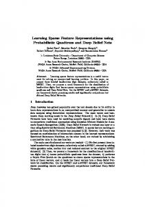
Figure 2. Results of PSR learning using non-blind policies as compared to blind random policies for three systems. Note that the error uses a logarithmic scale. See text for details.

program produces the policy variables π(h) for every history that is a prefix of some history-test pair. The policy can then be computed, Pr(a|h) =

π(hao) . π(h)

and used to gather data for the next iteration of the algorithm.

6. Results As mentioned earlier, existing PSR discovery and learning algorithms use blind policies, as opposed to our algorithm which computes and follows a non-blind policy. The following experiments evaluate the difference in performance between these two types of policies. The blind policy used for these experiments is the uniform-random policy, selecting each action with the same probability. In evaluating PSR discovery and learning algorithms, a common technique (James & Singh, 2004) is to include a reset, which is an additional action that brings the system to a fixed, but unknown, state. Existing work (Wolfe et al., 2005) shows how to extend discovery and learning algorithms to the more general case without reset. However, since our objective is just to evaluate the effect of blind and non-blind policies, our experiments include a reset.

We selected three dynamical systems that are commonly used in evaluating PSRs and POMDPs, whose definitions are available online (Cassandra, 1999). Our experimental method used the reset-based PSR discovery and learning algorithm (James & Singh, 2004), but used the above optimization to compute non-blind policies for action selection during exploration. A typical PSR discovery and learning run involves a number of iterations, each of which will identify specific histories and tests for which additional samples would be desirable. During each iteration, these sets of histories and tests are passed into the linear program, along with estimates of p(h) and #h, for appropriate h. The optimization is run five times for each iteration of discovery and learning, in order to maintain a reasonably current exploration policy. After the discovery and learning algorithm has completed (see James and Singh (2004) for details on the stopping condition), the resulting PSR model is evaluated. This is accomplished by running the model for a long sequence following the random policy, and computing the average one-step error. The error for a run is, L

1 XX 2 ˆ [Pr(o|ht at ) − Pr(o|h t at )] , L t=1 o∈O

where Pr(o|ht at ) is the true probability of observation o in

Learning Predictive State Representations Using Non-Blind Policies

history ht when the randomly selected action at is taken, ˆ and Pr(o|h t at ) is the corresponding prediction from the estimated model. For these experiments, L = 100, 000. This procedure tests all the parameters of the PSR model, not just the parameters for one-step prediction, because the update procedure, which is used L times, will require the use of all of the parameters. Results are presented in Figure 2, displaying data for a number of different discovery and learning runs for each system. The x-axis shows the amount of data used for a particular run, measured by the total number of sample trajectories. Each trajectory begins with the reset action and continues until the next reset is taken. The y-axis shows the error as defined above. Note that these graphs use a logarithmic scale, so small differences in the graphs correspond to order of magnitude improvements in test error. The test error when using the exploration policy in the paint domain is dramatically lower than when using the blind random exploration policy. The improvement is less dramatic in the tiger domain, but still amounts to a factor of two reduction in the amount of data needed to learn a model with equivalent accuracy. The exploration policy performs similarly to the random policy in the float-reset domain. This is not surprising since the the first few core-tests of the domain are both very easy to learn and are enough to attain fairly accurate predictions. In addition, it should be noted that the test error is measured while following the random policy, which may bias the results in favor of random exploration.

References Cassandra, A. (1999). Tony’s POMDP file repository page. http://www.cs.brown.edu/research/ai/pomdp/examples/. James, M. R., & Singh, S. (2004). Learning and discovery of predictive state representations in dynamical systems with reset. Proceedings of the 21st International Conference on Machine Learning (ICML) (pp. 719–726). Koller, D., Megiddo, N., & von Stengel, B. (1996). Efficient computation of equilibria for extensive two-person games. Games and Economic Behavior, 14, 247–259. Littman, M., Sutton, R. S., & Singh, S. (2002). Predictive representations of state. Advances in Neural Information Processing Systems 14 (NIPS) (pp. 1555–1561). MIT Press. McCracken, P., & Bowling, M. (2006). Online learning of predictive state representations. Advances in Neural Information Processing Systems 18 (NIPS). MIT Press. To appear. Rosencrantz, M., Gordon, G., & Thrun, S. (2004). Learning low dimensional predictive representations. Proceedings of the 21st International Conference on Machine Learning (ICML) (pp. 695–702). Singh, S., James, M. R., & Rudary, M. R. (2004). Predictive state representations: A new theory for modeling dynamical systems. Uncertainty in Artificial Intelligence: Proceedings of the Twentieth Conference (UAI) (pp. 512–519).

7. Conclusion The Monte Carlo estimator for predictions is integral to the majority of current algorithms for discovery and learning in PSRs. The problem, as proven in this paper, is that it is only an unbiased estimator when a blind policy is used to gather data. Simple examples demonstrate that this bias can be extreme depending on the policy. We provided a corrected Monte Carlo estimator that is unbiased for all policies, even when the policy is not known. We further provided a new variance-minimizing exploration algorithm and demonstrated its improvement over a blind policy exploration algorithm in common non-Markovian test domains.

Acknowledgments We would like to thank Peter Hooper for his initial observation of the inconsistency of Monte Carlo estimates. We would also like to thank Richard Sutton for numerous discussions. This work was partially funded by NSERC, iCore, and Alberta Ingenuity through the Alberta Ingenuity Centre for Machine Learning.

Singh, S., Littman, M., Jong, N., Pardoe, D., & Stone, P. (2003). Learning predictive state representations. Proceedings of the Twentieth International Conference on Machine Learning (ICML) (pp. 712–719). Wiewiora, E. (2005). Learning predictive representations from a history. Proceedings of the 22nd International Conference on Machine Learning (ICML) (pp. 969– 976). Wolfe, B., James, M. R., & Singh, S. (2005). Learning predictive state representations in dynamical systems without reset. Proceedings of the 22nd International Conference on Machine Learning (ICML) (pp. 985–992).