Learning Supervised PageRank with Gradient-Based and Gradient ...

1–34

Learning Supervised PageRank with Gradient-Based and Gradient-Free Optimization Methods Lev Bogolubsky

BOGOLUBSKY @ YANDEX - TEAM . RU

arXiv:1603.00717v1 [math.OC] 2 Mar 2016

Yandex, Leo Tolstoy st. 16, Moscow, Russian Federation

Pavel Dvurechensky PAVEL . DVURECHENSKY @ WIAS - BERLIN . DE Weierstrass Institute for Applied Analysis and Stochastics, Mohrenstr. 39, Berlin, Germany Institute for Information Transmission Problems RAS, Bolshoy Karetny per. 19, build.1, Moscow, Russian Federation Alexander Gasnikov

GASNIKOV @ YANDEX . RU Institute for Information Transmission Problems RAS, Bolshoy Karetny per. 19, build.1, Moscow, Russian Federation

Gleb Gusev

GLEB 57@ YANDEX - TEAM . RU

Yandex, Leo Tolstoy st. 16, Moscow, Russian Federation

Yurii Nesterov

YURII . NESTEROV @ UCLOUVAIN . BE

Center for Operations Research and Econometrics (CORE) 34 voie du Roman Pays, 1348, Louvain-la-Neuve, Belgium

Andrey Raigorodskii

RAIGORODSKY @ YANDEX - TEAM . RU

Yandex, Leo Tolstoy st. 16, Moscow, Russian Federation

Aleksey Tikhonov

ALTSOPH @ YANDEX - TEAM . RU

Yandex, Leo Tolstoy st. 16, Moscow, Russian Federation

Maksim Zhukovskii

ZHUKMAX @ YANDEX - TEAM . RU

Yandex, Leo Tolstoy st. 16, Moscow, Russian Federation

Abstract In this paper, we consider a non-convex loss-minimization problem of learning Supervised PageRank models, which can account for some properties not considered by classical approaches such as the classical PageRank model. We propose gradient-based and random gradient-free methods to solve this problem. Our algorithms are based on the concept of an inexact oracle and unlike the state state-of-the-art gradient-based method we manage to provide theoretically the convergence rate guarantees for both of them. In particular, under the assumption of local convexity of the loss function, our random gradient-free algorithm guarantees decrease of the loss function value expectation. At the same time, we theoretically justify that without convexity assumption for the loss function our gradient-based algorithm allows to find a point where the stationary condition is fulfilled with a given accuracy. For both proposed optimization algorithms, we find the settings of hyperparameters which give the lowest complexity (i.e., the number of arithmetic operations needed to achieve the given accuracy of the solution of the loss-minimization problem). The resulting estimates of the complexity are also provided. Finally, we apply proposed optimization algorithms to the web page ranking problem and compare proposed and state-of-the-art algorithms in terms of the considered loss function.

c L. Bogolubsky, P. Dvurechensky, A. Gasnikov, G. Gusev, Y. Nesterov, A. Raigorodskii, A. Tikhonov & M. Zhukovskii.

B OGOLUBSKY ET AL .

1. INTRODUCTION The most acknowledged methods of measuring importance of nodes in graphs are based on random walk models. Particularly, PageRank Page et al. (1999), HITS Kleinberg (1998), and their variants Haveliwala (1999, 2002); Richardson and Domingos (2002) are originally based on a discretetime Markov random walk on a link graph. According to the PageRank algorithm, the score of a node equals to its probability in the stationary distribution of a Markov process, which models a random walk on the graph. Despite undeniable advantages of PageRank and its mentioned modifications, these algorithms miss important aspects of the graph that are not described by its structure. In contrast, a number of approaches allows to account for different properties of nodes and edges between them by encoding them in restart and transition probabilities (see Dai and Davison (2010); Eiron et al. (2004); Gao et al. (2011); Jeh and Widom (2003); Liu et al. (2008); Zhukovskii et al. (2013a, 2014)). These properties may include, e.g., the statistics about users’ interactions with the nodes (in web graphs Liu et al. (2008) or graphs of social networks Backstrom and Leskovec (2011)), types of edges (such as URL redirecting in web graphs Zhukovskii et al. (2013a)) or histories of nodes’ and edges’ changes Zhukovskii et al. (2013b). Particularly, the transition probabilities in BrowseRank algorithm Liu et al. (2008) are proportional to weights of edges which are equal to numbers of users’ transitions. In the general ranking framework called Supervised PageRank Zhukovskii et al. (2014), weights of nodes and edges in a graph are linear combinations of their features with coefficients as the model parameters. The existing optimization method Zhukovskii et al. (2014) of learning these parameters and the optimizations methods proposed in the presented paper have two levels. On the lower level, the following problem is solved: to estimate the value of the loss function (in the case of zero-order oracle) and its derivatives (in the case of first-order oracle) for a given parameter vector. On the upper level, the estimations obtained on the lower level of the optimization methods (which we also call inexact oracle information) are used for tuning the parameters by an iterative algorithm. Following Gao et al. (2011), the authors of Supervised PageRank consider a non-convex loss-minimization problem for learning the parameters and solve it by a two-level gradient-based method. On the lower level of this algorithm, an estimation of the stationary distribution of the considered Markov random walk is obtained by classical power method and estimations of derivatives w.r.t. the parameters of the random walk are obtained by power method introduced in Andrew (1978, 1979). On the upper level, the obtained gradient of the stationary distribution is exploited by the gradient descent algorithm. As both power methods give imprecise values of the stationary distribution and its derivatives, there was no proof of the convergence of the state-of-the-art gradient-based method to a local optimum (for locally convex loss functions) or to the stationary point (for not locally convex loss functions). The considered constrained non-convex loss-minimization problem from Zhukovskii et al. (2014) can not be solved by existing optimization methods which require exact values of the objective function such as Nesterov and Spokoiny (2015) and Ghadimi and Lan (2014) due to presence of constraints for parameter vector and the impossibility to calculate exact value of the loss function and its gradient. Moreover, standard global optimization methods can not be applied to solve it, because they need access to some stochastic approximation for the loss-function value which in expectation coincides with the true value of the loss-function. In our paper, we propose two two-level methods to solve the loss-minimization problem from Zhukovskii et al. (2014). On the lower level of these methods, we use the linearly convergent method from Nes-

2

L EARNING S UPERVISED PAGE R ANK

terov and Nemirovski (2015) to calculate an approximation to the stationary distribution of Markov random walk. We analyze other methods from Gasnikov and Dmitriev (2015) and show that the chosen method is the most suitable since it allows to approximate the value of the loss function with any given accuracy and has lowest complexity estimation among others. Upper level of the first method is gradient-based. The main obstacle which we have overcome is that the state-of-the-art methods for constrained non-convex optimization assume that the gradient is known exactly, which is not the case in our problem. We develop a gradient method for general constrained non-convex optimization problems with inexact oracle, estimate its convergence rate to the stationary point of the problem. One of the advantages of our method is that it does not require to know the Lipschitz-constant of the gradient of the goal function, which is usually used to define the stepsize of a gradient algorithm. In order to calculate approximation of the gradient which is used in the upper-level method, we generalize linearly convergent method from Nesterov and Nemirovski (2015) (and use it as part of the lower-level method). We prove that it has a linear rate of convergence as well. Upper level of our second method is random gradient-free. Like for the gradient-based method, we encounter the problem that the existing gradient-free optimization methods Ghadimi and Lan (2014); Nesterov and Spokoiny (2015) require exact values of the objective function. Our contribution to the gradient-free methods framework consists in adapting the approach of Nesterov and Spokoiny (2015) to the case when the value of the function is calculated with some known accuracy. We prove a convergence theorem for this method and exploit it on the upper level of the two-level algorithm for solving the problem of learning Supervised PageRank. Another contribution consists in investigating both for the gradient and gradient-free methods the trade-off between the accuracy of the lower-level algorithm, which is controlled by the number of iterations of method in Nesterov and Nemirovski (2015) and its generalization (for derivatives estimation), and the computational complexity of the two-level algorithm as a whole. Finally, we estimate the complexity of the whole two-level algorithms for solving the loss-minimization problem with a given accuracy. In the experiments, we apply our algorithms to learning Supervised PageRank on real data (we consider the problem of web pages’ ranking). We show that both two-level methods outperform the state-of-the-art gradient-based method from Zhukovskii et al. (2014) in terms of the considered loss function. Summing up, apart from the state-of-the-art method our algorithms have theoretically proven estimates of convergence rate and outperform it in the ranking quality (as we prove experimentally). The main advantages of the first gradient-based algorithm are the following. There is no need to assume that the function is locally convex in order to guarantee that it converges to the stationary point. This algorithm has smaller number of input parameters than gradient-free, because it does not need the Lipschitz constant of the gradient of the loss function. The main advantage of the second gradient-free algorithm is that it avoids calculating the derivative for each element of a large matrix. The remainder of the paper is organized as follows. In Section 2, we describe the random walk model. In Section 3, we define the loss-minimization problem and discuss its properties. In Section 4, we state two technical lemmas about the numbers of iterations of Nesterov–Nemirovski method (and its generalization) needed to achieve any given accuracy of the loss function (and its gradient). In Section 5 and Section 6 we describe the framework of random gradient-free and gradient-based optimization methods respectively, generalize them to the case when the objective function values and gradients are inaccurate and propose two-level algorithms for the stated loss3

B OGOLUBSKY ET AL .

minimization problem. Proofs of all our results can be found in Appendix. The experimental results are reported in Section 7. In Section 8, we summarize the outcomes of our study, discuss its benefits and directions of future work.

2. MODEL DESCRIPTION Let Γ = (V, E) be a directed graph. Let F1 = {F (ϕ1 , ·) : V → R}, F2 = {G(ϕ2 , ·) : E → R} be two classes of functions parametrized by ϕ1 ∈ Rm1 , ϕ2 ∈ Rm2 respectively, where m1 is the number of nodes’ features, m2 is the number of edges’ features. As in Zhukovskii et al. (2014), we 1 suppose that for any i ∈ V and any ˜i → i ∈ E, a vector of node’s features Vi ∈ Rm + and a vector m2 of edge’s features E˜ii ∈ R+ are given. We set G(ϕ1 , ˜i → i) = hϕ2 , E˜ii i.

F (ϕ1 , i) = hϕ1 , Vi i,

(2.1)

We denote m = m1 + m2 , p = |V |. Let us describe the random walk on the graph Γ, which was considered in Zhukovskii et al. (2014). A surfer starts a random walk from a random page i ∈ U (U is some subsetP in V called seed set, |U | = n). We assume that ϕ1 and node features are chosen in such way that ˜i∈U F (ϕ1 , ˜i) is non-zero. The initial probability of being at vertex i ∈ V is called the restart probability and equals F (ϕ1 , i) , ˜ ˜i∈U F (ϕ1 , i)

[π 0 (ϕ)]i = P

i∈U

(2.2)

and [π 0 (ϕ)]i = 0 for i ∈ V \ U . At each step, the surfer (with a current position ˜i ∈ V ) either chooses with probability α ∈ (0, 1) (originally Page et al. (1999), α = 0.15), which is called the damping factor, to go to any vertex from V in accordance with the distribution π 0 (ϕ) (makes a restart) or chooses to traverse an outgoing edge (makes a transition) P with probability 1 − α. We assume that ϕ2 and edges features are chosen in such way that j:˜i→j G(ϕ2 , ˜i → j) is non-zero for all ˜i with non-zero outdegree. For ˜i with non-zero outdegree, the probability G(ϕ2 , ˜i → i) ˜ j:˜i→j G(ϕ2 , i → j)

[P (ϕ)]˜i,i = P

(2.3)

of traversing an edge ˜i → i ∈ E is called the transition probability. If an outdegree of ˜i equals 0, then we set [P (ϕ)]˜i,i = [π 0 (ϕ)]i for all i ∈ V (the surfer with current position ˜i makes a restart with probability 1). Finally, by Equations 2.2 and 2.3 the total probability of choosing vertex i ∈ V conditioned by the surfer being at vertex ˜i equals α[π 0 (ϕ)]i + (1 − α)[P (ϕ)]˜i,i . Denote by π ∈ Rp the stationary distribution of the described Markov process. It can be found as a solution of the system of equations X [π]i = α[π 0 (ϕ)]i + (1 − α) [P (ϕ)]˜i,i [π]˜i . (2.4) ˜i:˜i→i∈E

In this paper, we learn the ranking algorithm, which orders the vertices i by their probabilities [π]i in the stationary distribution π. 4

L EARNING S UPERVISED PAGE R ANK

3. LOSS-MINIMIZATION PROBLEM STATEMENT Let Q be a set of queries and, for any q ∈ Q, a set of nodes Vq which are relevant to q be given. We are also provided with a ranking algorithm which assigns nodes ranking scores [πq ]i , i ∈ Vq , πq = πq (ϕ), as its output. For example, in web search, the score [πq ]i may repesent relevance of the page i w.r.t. the query q. Our goal is to find the parameter vector ϕ which minimizes the discrepancy of the ranking scores from the ground truth scoring defined by assessors. For each q ∈ Q, there is a set of nodes in Vq manually judged and grouped by relevance labels 1, . . . , k. We denote Vqj the set of documents annotated with label k +1−j (i.e., Vq1 is the set of all nodes with the highest relevance score). For any two nodes i1 ∈ Vqj1 , i2 ∈ Vqj2 , let h(j1 , j2 , [πq ]i2 − [πq ]i1 ) be the value of the loss function. If it is non-zero, then the position of the node i1 according to our ranking algorithm is higher than the position of the node i2 but j1 > j2 . We consider square loss with margins bj1 j2 ≥ 0, where 1 ≤ j2 < j1 ≤ k: h(j1 , j2 , x) = (min{x + bj1 j2 , 0})2 as it was done in previous studies Liu et al. (2008); Zhukovskii et al. (2014, 2013b). Finally, we minimize |Q|

1 X |Q|

X

X

h(j1 , j2 , [πq ]i2 − [πq ]i1 )

(3.1)

q=1 1≤j2 0 such that the set Φ (which we call the feasible set of parameters) defined as Φ = {ϕ ∈ Rm : kϕ − ϕk ˆ 2 ≤ R} lies in m 1 the set of vectors with positive components R++ . We denote by πq (ϕ) the solution of the equation πq = απq0 (ϕ) + (1 − α)PqT (ϕ)πq

(3.2)

which is Equation (2.4) rewritten for fixed q ∈ Q in the vector form. From (3.2) we obtain the dπq (ϕ) following equation for pq × m matrix dϕ which is the derivative of stationary distribution πq (ϕ) T 1. As probablities [πq0 (ϕ)]i , i ∈ Vq , [Pq (ϕ)]˜i,i , ˜i → i ∈ Eq , are scale-invariant (πq0 (λϕ) = πq0 (ϕ), Pq (λϕ) = Pq (ϕ)), in our experiments, we consider the set Φ = {ϕ ∈ Rm : kϕ − em k2 ≤ 0.99} , where em ∈ Rm is the vector of all ones, that has large intersection with the simplex {ϕ ∈ Rm ++ : kϕk1 = 1}

5

B OGOLUBSKY ET AL .

with respect to ϕ dπq (ϕ) dπq (ϕ) = Π0q (ϕ) + (1 − α)PqT (ϕ) , T dϕ dϕT where

(3.3)

p

Π0q (ϕ)

q X dπq0 (ϕ) dpi (ϕ) =α + (1 − α) [πq (ϕ)]i dϕT dϕT

(3.4)

i=1

and pi (ϕ) is the i-th column of the matrix PqT (ϕ). Let us rewrite the function defined in (3.1) as |Q|

f (ϕ) =

1 X k(Aq πq (ϕ) + bq )+ k22 , |Q|

(3.5)

q=1

where vector x+ has components [x+ ]i = max{xi , 0}, the matrices Aq ∈ Rrq ×pq , q ∈ Q represent assessor’s view of the relevance of pages to the query q, vectors bq , q ∈ Q are vectors composed from thresholds bj1 ,j2 in (3.1) with fixed q, rq is the number of summands in (3.1) with fixed q. We denote r = maxq∈Q rq . Then the gradient of the function f (ϕ) is easy to derive: |Q|

2 X ∇f (ϕ) = |Q| q=1



dπq (ϕ) dϕT

T

ATq (Aq πq (ϕ) + bq )+ .

(3.6)

Finally, the loss-minimization problem which we solve in this paper is as follows min f (ϕ), Φ = {ϕ ∈ Rm : kϕ − ϕk ˆ 2 ≤ R}. ϕ∈Φ

(3.7)

To solve this problem, we use gradient-free methods which are based only on f (ϕ) calculations (zero-order oracle) and gradient methods which are based on f (ϕ) and ∇f (ϕ) calculations (firstorder oracle). We do not use methods with oracle of higher order since the loss function is not convex and we assume that m is large.

4. NUMERICAL CALCULATION OF THE VALUE AND THE GRADIENT OF f (ϕ) One of the main difficulties in solving Problem 3.7 is that calculation of the value of the function f (ϕ) requires to calculate |Q| vectors πq (ϕ) which solve (3.2). In our setting, this vector has huge dimension pq and hence it is computationally very expensive to find it exactly. Moreover, in order to calculate ∇f (ϕ) one needs to calculate the derivative for each of these huge-dimensional vectors which is also computationally very expensive to be done exactly. At the same time our ultimate goal is to provide methods for solving Problem 3.7 with estimated rate of convergence and complexity. Due to the expensiveness of calculating exact values of f (ϕ) and ∇f (ϕ) we have to use the framework of optimization methods with inexact oracle which requires to control the accuracy of the oracle, otherwise the convergence is not guaranteed. This means that we need to be able to calculate an approximation to the function f (ϕ) value (inexact zero-order oracle) with a given accuracy for gradient-free methods and approximation to the pair (f (ϕ), ∇f (ϕ)) (inexact first-order 6

L EARNING S UPERVISED PAGE R ANK

oracle) with a given accuracy for gradient methods. Hence we need some numerical scheme which dπq (ϕ) allows to calculate approximation for πq (ϕ) and dϕ for every q ∈ Q with a given accuracy. T Motivated by the last requirement we have analysed state-of-the-art methods for finding the solution of Equation 3.2 in huge dimension summarized in the review Gasnikov and Dmitriev (2015) and power method, used in Page et al. (1999); Backstrom and Leskovec (2011); Zhukovskii et al. (2014). Only four methods allow to make the difference kπq (ϕ) − π ˜q k, where π ˜q is the approximation, small for some norm k · k which is crucial to estimate the error in the approximation of the function f (ϕ) value. These method are: Markov Chain Monte Carlo (MCMC), Spillman’s, Nesterov-Nemirovski’s (NN) and power method. Spillman’s algoritm and power method converge in infinity norm which is usually pq times larger than 1-norm. MCMC converges in 2-norm which √ is usually pq times larger than 1-norm. Also MCMC is randomized and converges only in average which makes it hard to control the accuracy of the approximation π ˜q . Apart from the other three, √ NN is deterministic and converges in 1-norm which gives minimum pq times better approximation. At the same time, to the best of our knowledge, NN method is the only method that admits dπq (ϕ) a generalization which, as we prove in this paper, calculates the derivative dϕ with any given T accuracy. The method by Nesterov and Nemirovski (2015) for approximation of πq (ϕ) for any fixed q ∈ Q constructs a sequence πk by the following rule π0 = πq0 (ϕ),

πk+1 = PqT (ϕ)πk .

(4.1)

The output of the algorithm (for some fixed non-negative integer N ) is π ˜qN (ϕ) =

N X α (1 − α)k πk . 1 − (1 − α)N +1

(4.2)

k=0

Lemma 1 Assume that for some δ1 > 0 Method 4.1, 4.2 with N =

l

1 α

m ln 8r δ1 −1 is used to calculate

the vector π ˜qN (ϕ) for every q ∈ Q. Then |Q|

1 X f˜(ϕ, δ1 ) = k(Aq π ˜qN (ϕ) + bq )+ k22 |Q|

(4.3)

|f˜(ϕ, δ1 ) − f (ϕ)| ≤ δ1 .

(4.4)

q=1

satisfies Moreover, the calculation of f˜(ϕ, δ1 ) requires not more than |Q|(3mps + 3psN + 6r) a.o. The proof of Lemma 1 can be found in Appendix A.1. dπq (ϕ) Our generalization of the method Nesterov and Nemirovski (2015) for calculation of dϕ for T N 1 any q ∈ Q is the following. Choose some non-negative integer N1 and calculate π ˜q (ϕ) using (4.1), (4.2). Start with initial point p

q X dπq0 (ϕ) dpi (ϕ) N1 Π0 = α + (1 − α) [˜ πq (ϕ)]i . dϕT dϕT

i=1

7

(4.5)

B OGOLUBSKY ET AL .

Iterate Πk+1 = PqT (ϕ)Πk .

(4.6)

The output is (for some fixed non-negative integer N2 ) 2 ˜N Π q (ϕ) =

N2 X 1 (1 − α)k Πk . 1 − (1 − α)N2 +1

(4.7)

k=0

n1 ×n2 : kAk = In what follows, 1 Pn1 we use the following norm on the space of matrices A ∈ R maxj=1,...,n2 i=1 |aij |.

Lemma 2 Let β1 be a number (explicitly computable, see Appendix A.2 Equation A.11) such that for all ϕ ∈ Φ

pq

dπ 0 (ϕ) X

dpi (ϕ)

q

0

kΠq (ϕ)k1 ≤ α (4.8)

+ (1 − α)

dϕT ≤ β1 .

dϕT i=1

1

l

1

m

1r ln 24β − 1 is used for every q ∈ Q to calculate the αδ2 m l 1r vector π ˜qN1 (ϕ) (4.2) and Method 4.5, 4.6, 4.7 with N2 = α1 ln 8β αδ2 − 1 is used for every q ∈ Q to 2 ˜N calculate the matrix Π q (ϕ) (4.7). Then the vector

Assume that Method 4.1, 4.2 with N1 =

1 α

|Q|

g˜(ϕ, δ2 ) =

T 2 X  ˜ N2 Πq (ϕ) ATq (Aq π ˜qN1 (ϕ) + bq )+ |Q|

(4.9)

q=1

satisfies k˜ g (ϕ, δ2 ) − ∇f (ϕ)k∞ ≤ δ2 .

(4.10)

Moreover the calculation of g˜(ϕ, δ2 ) requires not more than |Q|(10mps + 3psN1 + 3mpsN2 + 7r) a.o. The proof of Lemma 2 can be found in Appendix A.2.

5. RANDOM GRADIENT-FREE OPTIMIZATION METHODS In this section, we first describe general framework of random gradient-free methods with inexact oracle and then apply it for Problem 3.7. Lemma 1 allows to control the accuracy of the inexact zero-order oracle and hence apply random gradient-free methods with inexact oracle. 5.1. GENERAL FRAMEWORK Below we extend the framework of random gradient-free methods Agarwal et al. (2010); Nesterov and Spokoiny (2015); Ghadimi and Lan (2014) for the situation of presence of uniformly bounded error of unknown nature in the value of an objective function in general optimization problem. Apart from Nesterov and Spokoiny (2015), we consider a randomization on a Euclidean sphere which seems to give better large deviations bounds and doesn’t need the assumption that the objective function can be calculated at any point of Rm .

8

L EARNING S UPERVISED PAGE R ANK

Let E be a m-dimensional vector space. In this subsection, we consider a general function f (·) : E → R and denote its argument by x or y to avoid confusion with other sections. We choose some norm k · k in E and say that f ∈ CL1,1 (k · k) iff |f (x) − f (y) − h∇f (y), x − yi| ≤

L kx − yk2 , 2

∀x, y ∈ E.

(5.1)

The problem of our interest is to find minx∈X f (x), where f ∈ CL1,1 (k · k), X is a closed convex set and there exists a number D ∈ (0, +∞) such that diamX := maxx,y∈X kx − yk ≤ D. Also ˜ we assume that the inexact zero-order oracle for f (x) returns a value f˜(x, δ) = f (x) + δ(x), where ˜ ˜ δ(x) is the error satisfying for some δ > 0 (which is known) |δ(x)| ≤ δ for all x ∈ X. Let x∗ ∈ arg minx∈X f (x). Denote f ∗ = minx∈X f (x). Apart from Nesterov and Spokoiny (2015), we define the biased gradient-free oracle m gµ (x, δ) = (f˜(x + µξ, δ) − f˜(x, δ))ξ, µ where ξ is a random vector uniformly distributed over the unit sphere S = {t ∈ Rm : ktk2 = 1}, µ is a smoothing parameter. Algorithm 1 below is the variation of the gradient descent method. Here ΠX (x) denotes the Euclidean projection of a point x onto the set X. Algorithm 1 Gradient-type method Input: Point x0 ∈ X, stepsize h > 0, number of steps M . Set k = 0. repeat Generate ξk and calculate corresponding gµ (xk , δ). Calculate xk+1 = ΠX (xk − hgµ (xk , δ)). Set k = k + 1. until k > M Output: The point x ˆM = arg minx {f (x) : x ∈ {x0 , . . . , xM }}. Next theorem gives the convergence rate of Algorithm 1. Denote by Uk = (ξ0 , . . . , ξk ) the history of realizations of the vector ξ generated on each iteration of the algorithm. Theorem 1 Let f ∈ CL1,1 (k · k2 ) and convex. Assume that x∗ ∈ intX, and the sequence xk is 1 generated by Algorithm 1 with h = 8mL . Then for any M ≥ 0, we have EUM −1 f (ˆ xM ) − f ∗ ≤ ≤

8mLD2 µ2 L(m + 8) δmD δ 2 m + + + . M +1 8 4µ Lµ2

(5.2)

The full proof of the theorem is in Appendix B. It is easy to see that to make the right hand side of (5.2) less than a desired accuracy ε it is sufficient to choose s   3√ 32mLD2 2ε ε2 2 p M= , µ= , δ≤ . (5.3) ε L(m + 8) 8mD L(m + 8) 9

B OGOLUBSKY ET AL .

5.2. SOLVING THE LEARNING PROBLEM In this subsection, we apply the results of the previous subsection to solve Problem 3.7 in the following way. We assume that the set Φ is a small vicinity of some local minimum ϕ∗ and the function f (ϕ) is convex in this vicinity (generally speaking, the function defined in (3.5) is nonconvex). We choose the desired accuracy ε for approximation of the optimal value f ∗ in this problem. This accuracy in accordance with (5.3) gives us the number of steps of Algorithm 1, the value of the parameter µ, the value of the required accuracy δ of the inexact zero-order oracle. Knowing the value δ, using Lemma 1 we choose the number of steps N of Algorithm 4.1, 4.2 and calculate an approximation f˜(ϕ, δ) for the function f (ϕ) value with accuracy δ. Then we use the inexact zeroorder oracle f˜(ϕ, δ) to make a step of Algorithm 1. Theorem 1 and the fact that the feasible set Φ is a Euclidean ball makes it natural to choose k · k2 -norm in the space Rm of parameter ϕ. It is easy to see that in this norm diamΦ ≤ 2R. Algorithm 2 is a formal record of these ideas. To the best of our knowledge, this is the first time when the idea of random gradient-free optimization methods is combined with some efficient method for huge-scale optimization using the concept of an inexact zero-order oracle. Algorithm 2 Gradient-free method for Problem 3.7 Input: Point ϕ0 ∈ Φ, L – Lipschitz constant for the function f (ϕ) on Φ, accuracy ε > 0. l m q 3√ 2 2 2 ε√ 2ε Define M = 128m LR , µ = , δ = ε L(m+8) . 16mR

L(m+8)

Set k = 0. repeat Generate random vector ξk uniformly distributed over a unit Euclidean sphere S in Rm . Calculate f˜(ϕk + µξk , δ), f˜(ϕk , δ) using Lemma 1 with δ1 = δ. ˜ ˜ Calculate gµ (ϕk , δ) = m µ (f (ϕk + µξk , δ) −
f (ϕk , δ))ξk . 1 Calculate ϕk+1 = ΠΦ ϕk − 8mL gµ (ϕk , δ) . Set k = k + 1. until k > M Output: The point ϕˆM = arg minϕ {f (ϕ) : ϕ ∈ {ϕ0 , . . . , ϕM }}. The most computationally hard on each iteration of the main cycle of this method are calculations of f˜(ϕk + µξk , δ), f˜(ϕk , δ). Using Lemma 1, we obtain that each iteration of Algorithm 2 needs not more than ! p 3ps 128mrR L(m + 8) √ 2|Q| 3mps + ln + 6r α ε3/2 2 a.o. So, we obtain the following result, which gives the complexity of Algorithm 2. Theorem 2 Assume that the set Φ in (3.7) is chosen in a way such that f (ϕ) is convex on Φ and some ϕ∗ ∈ arg minϕ∈Φ f (ϕ) belongs also to intΦ. Then the mean total number of arithmetic operations of the Algorithm 2 for the accuracy ε (i.e. for the inequality EUM −1 f (ϕˆM ) − f (ϕ∗ ) ≤ ε to hold) is not more than ! p LR2 1 128mrR L(m + 8) √ 768mps|Q| m + ln + 6r . ε α ε3/2 2

10

L EARNING S UPERVISED PAGE R ANK

6. GRADIENT-BASED OPTIMIZATION METHODS In this section, we first develop a general framework of gradient methods with inexact oracle for non-convex problems from rather general class and then apply it for the particular Problem 3.7. Lemma 1 and Lemma 2 allow to control the accuracy of the inexact first-order oracle and hence apply proposed framework. 6.1. GENERAL FRAMEWORK In this subsection, we generalize the approach in Ghadimi and Lan (2014) for constrained nonconvex optimization problems. Our main contribution consists in developing this framework for an inexact first-order oracle and unknown ”Lipschitz constant” of this oracle. Let E be a finite-dimensional real vector space and E ∗ be its dual. We denote the value of linear function g ∈ E ∗ at x ∈ E by hg, xi. Let k · k be some norm on E, k · k∗ be its dual. Our problem of interest in this subsection is a composite optimization problem of the form min{ψ(x) := f (x) + h(x)}, x∈X

(6.1)

where X ⊂ E is a closed convex set, h(x) is a simple convex function, e.g. kxk1 . We assume that f (x) is a general function endowed with an inexact first-order oracle in the following sense. There exists a number L ∈ (0, +∞) such that for any δ ≥ 0 and any x ∈ X one can calculate f˜(x, δ) ∈ R and g˜(x, δ) ∈ E ∗ satisfying L |f (y) − (f˜(x, δ) − h˜ g (x, δ), y − xi)| ≤ kx − yk2 + δ. 2

(6.2)

for all y ∈ X. The constant L can be considered as ”Lipschitz constant” because for the exact firstorder oracle for a function f ∈ CL1,1 (k · k) Inequality 6.2 holds with δ = 0. This is a generalization of the concept of (δ, L)-oracle considered in Devolder et al. (2013) for convex problems. We choose a prox-function d(x) which is continuously differentiable and 1-strongly convex on X with respect to k · k. This means that for any x, y ∈ X 1 d(y) − d(x) − h∇d(x), y − xi ≥ ky − xk2 . 2

(6.3)

We define also the corresponding Bregman distance: V (x, z) = d(x) − d(z) − h∇d(z), x − zi. Let us define for any x ¯ ∈ E, g ∈ E ∗ , γ > 0   1 ¯) + h(x) , xX (¯ x, g, γ) = arg min hg, xi + V (x, x x∈X γ gX (¯ x, g, γ) =

1 (¯ x − xX (¯ x, g, γ)). γ

(6.4)

(6.5) (6.6)

We assume that the set X is simple in a sense that the vector xX (¯ x, g, γ) can be calculated explicitly or very efficiently for any x ¯ ∈ X, g ∈ E ∗ , γ.

11

B OGOLUBSKY ET AL .

Algorithm 3 Adaptive projected gradient algorithm Input: Point x0 ∈ X, number L0 > 0. Set k = 0, z = +∞. repeat Set Mk = Lk , flag = 0. repeat ε Set δ = 16M . k Calculate f˜(xk , δ) and g˜(xk , δ). Find   1 wk = xX xk , g˜(xk , δ), Mk

(6.7)

Calculate f˜(wk , δ). If the inequality f˜(wk , δ) ≤ f˜(xk , δ) + h˜ g (xk , δ), wk − xk i+ Mk ε + kwk − xk k2 + 2 8Mk

(6.8)

holds, set flag = 1. Otherwise set Mk = 2Mk . until flag = 1 Mk Set xk+1  = 2 , g˜k = g˜ (xk ,δ).   = wk , Lk+1

1 1 ˆ If gX xk , g˜k , Mk < z, set z = gX xk , g˜k , Mk , k = k. Set k = k + 1. until z ≤ ε Output: The point xk+1 ˆ . Theorem 3 Assume that f (x) is endowed with the inexact first-order oracle in a sense (6.2) and that there exists a number ψ ∗ > −∞ such that ψ(x) ≥ ψ ∗ for all x ∈ X. Then after M iterations of Algorithm 3 it holds that

  2 ∗

gX xˆ , g˜ˆ , 1 ≤ 4L(ψ(x0 ) − ψ ) + ε . (6.9)

k k M M +1 2 ˆ k Moreover, the total number of checks of Inequality 6.8 is not more than M + log2

2L L0 .

The full proof of the theorem is in Appendix C.   2

It is easy to show that when gX xkˆ , g˜kˆ , M1ˆ ≤ ε for small ε, then for all x ∈ X it holds k D E √ that ∇f (xk+1 ≥ −c ε, where c > 0 is a constant, p is some subgradient of ˆ ) + p, x − xk+1 ˆ h(x) at xk+1 the necessary condition of a local minimum is ˆ . This means that at the point xk+1 ˆ fulfilled with a good accuracy, i.e. xk+1 is a good approximation of a stationary point. ˆ

12

L EARNING S UPERVISED PAGE R ANK

6.2. SOLVING THE LEARNING PROBLEM In this subsection, we return to Problem 3.7 and apply the results of the previous subsection. For √ this problem, h(·) ≡ 0. It is easy to show that in 1-norm diamΦ ≤ 2R m. For any δ > 0, Lemma 1 with δ1 = 2δ allows us to obtain f˜(ϕ, δ1 ) such that Inequality 4.4 holds and Lemma 2 with δ2 = 4Rδ√m allows us to obtain g˜(ϕ, δ2 ) such that Inequality 4.10 holds. Similar to Devolder et al. (2013), since f ∈ CL1,1 (k · k2 ), these two inequalities lead to Inequality 6.2 for f˜(ϕ, δ1 ) in the role of f˜(x, δ), g˜(ϕ, δ2 ) in the role of g˜(x, δ) and k · k2 in the role of k · k. We choose the desired accuracy ε for approximating the stationary point of Problem 3.7. This accuracy gives the required accuracy δ of the inexact first-order oracle for f (ϕ) on each step of the inner cycle of the Algorithm 3. Knowing the value δ1 = 2δ and using Lemma 1, we choose the number of steps N of Algorithm 4.1, 4.2 and thus approximate f (ϕ) with the required accuracy δ1 by f˜(ϕ, δ1 ). Knowing the value δ2 = 4Rδ√m and using Lemma 2, we choose the number of steps N1 of Algorithm 4.1, 4.2 and the number of steps N2 of Algorithm 4.5, 4.6, 4.7 and obtain the approximation g˜(ϕ, δ2 ) of ∇f (ϕ) with the required accuracy δ2 . Then we use the inexact first-order oracle (f˜(ϕ, δ1 ), g˜(ϕ, δ2 )) to perform a step of Algorithm 3. Since Φ is the Euclidean ball, it is natural to set E = Rm and k · k = k · k2 , choose the prox-function d(ϕ) = 12 kϕk22 . Then the Bregman distance is V (ϕ, ω) = 21 kϕ − ωk22 . Algorithm 4 is a formal record of the above ideas. To the best of our knowledge, this is the first time when the idea of gradient optimization methods is combined with some efficient method for huge-scale optimization using the concept of an inexact first-order oracle. The most computationally consuming operations of the inner cycle of Algorithm 4 are calculations of f˜(ϕk , δ1 ), f˜(ωk , δ1 ) and g˜(ϕk , δ2 ). Using Lemma 1 and Lemma 2, we obtain that each inner iteration of Algorithm 4 needs not more than √ 6mps|Q| 1024β1 rRL m 7r|Q| + ln α αε a.o. Using Theorem 3, we obtain the following result, which gives the complexity of Algorithm 4. Theorem 4 The number of arithmetic operations in Algorithm 4 for the accuracy ε (i.e. for

total  2 

the inequality gΦ ϕkˆ , g˜(ϕkˆ δ2 ), M1ˆ ≤ ε to hold) is not more than k



2

2L 8L(f (ϕ0 ) − f ∗ ) + log2 ε L0

 √  6mps|Q| 1024β1 rRL m 7r|Q| + ln . α αε

7. EXPERIMENTAL RESULTS We apply different learning techniques, our gradient-free and gradient-based methods and state-ofthe-art gradient-based method, to the web page ranking problem and compare their performances. In the next section, we describe the graph, which we exploit in our experiments (the user browsing graph). In Section 7.2 and Section 7.3, we describe the dataset and the results of the experiments respectively.

13

B OGOLUBSKY ET AL .

Algorithm 4 Adaptive gradient method for Problem 3.7 Input: Point ϕ0 ∈ Φ, number L0 > 0, accuracy ε > 0. Set k = 0, z = +∞. repeat Set Mk = Lk , flag = 0. repeat ε Set δ1 = 32M , δ2 = 64M εR√m . k k Calculate f˜(ϕk , δ1 ) using Lemma 1 and g˜(ϕk , δ2 ) using Lemma 2. Find

  Mk 2 g (ϕk , δ2 ), ϕi + ωk = arg min h˜ kϕ − ϕk k2 . ϕ∈Φ 2

Calculate f˜(ωk , δ1 ) using Lemma 1. If the inequality ε Mk kωk − ϕk k22 + f˜(ωk , δ1 ) ≤ f˜(ϕk , δ1 ) + h˜ g (ϕk , δ2 ), ωk − ϕk i + 2 8Mk holds, set flag = 1. Otherwise set Mk = 2Mk . until flag = 1 Mk Set ϕk+1 2 ,.

  = ωk , Lk+1 =  

1 If gΦ ϕk , g˜(ϕk , δ2 ), Mk < z, set z = gΦ ϕk , g˜(ϕk , δ2 ), M1k , kˆ = k. 2 2 Set k = k + 1. until z ≤ ε Output: The point ϕk+1 ˆ . 7.1. USER BROWSING GRAPH In this section, we define the user web browsing graph (which was first considered in Liu et al. (2008)). We choose the user browsing graph instead of a link graph with the purpose to make the model query-dependent. Let q be any query from the set Q. A user session Sq (see Liu et al. (2008)), which is started from q, is a sequence of pages (i1 , i2 , ..., ik ) such that, for each j ∈ {1, 2, ..., k − 1}, the element ij is a web page and there is a record ij → ij+1 which is made by toolbar. The session finishes if the user types a new query or if more than 30 minutes left from the time of the last user’s activity. We call pages ij , ij+1 , j ∈ {1, . . . , k − 1}, the neighboring elements of the session Sq . We define user browsing graphs Γq = (Vq , Eq ), q ∈ Q, as follows. The set of vertices Vq consists of all the distinct elements from all the sessions which are started from a query q ∈ Q. The set of directed edges Eq represents all the ordered pairs of neighboring elements (˜i, i) from such sessions. We add a page i in the seed set Uq if and only if there is a session which is started from q and contains i as its first element. Moreover, we set ˜i → i ∈ Eq if and only if there is a session which is started from q and contains the pair of neighboring elements ˜i, i.

14

L EARNING S UPERVISED PAGE R ANK

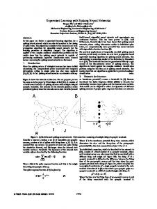
7.2. DATA All experiments are performed with pages and links crawled by a popular commercial search engine. We randomly choose the set of queries Q the user sessions start from, which contains 600 queries. There are ≈ 11.7K vertices and ≈ 7.5K edges in graphs Γq , q ∈ Q, in total. For each query, a set of pages was judged by professional assessors hired by the search engine. Our data contains ≈ 1.7K judged query–document pairs. The relevance score is selected from among 5 labels. We divide our data into two parts. On the first part Q1 (50% of the set of queries Q) we train the parameters and on the second part Q2 we test the algorithms. To define weights of nodes and edges we consider a set of m1 = 26 query–document features. For any q ∈ Q and i ∈ Vq , the vector Viq contains values of all these features for query–document pair (q, i). The vector of m2 = 52 features E˜qii for an edge ˜i → i ∈ Eq is obtained simply by concatenation of the feature vectors of pages ˜i and i. To study a dependency between the efficiency of the algorithms and the sizes of the graphs, we sort the sets Q1 , Q2 in ascending order of sizes of the respective graphs. Sets Q1j , Q2j , Q3j contain first (in terms of these order) 100, 200, 300 elements respectively for j ∈ {1, 2}. 7.3. PERFORMANCES OF THE OPTIMIZATION ALGORITHMS We find the optimal values of the parameters ϕ by all the considered methods (our gradient-free method GFN (Algorithm 2), the gradient-based method GBN (Algorithm 4), the state-of-the-art gradient-method GBP), which solve Problem 3.5. The sets of hyperparameters which are exploited by the optimization methods (and not tuned by them) are the following: the Lipschitz constant L = 10−4 in GFN (and L0 = 10−4 in GBN), the accuracy ε = 10−6 (in both GBN and GFN), the radius R = 0.99 (in both GBN and GFN). On all sets of queries, we compare final values of the loss function for GBN when L0 ∈ {10−4 , 10−3 , 10−2 , 10−1 , 1}. The differences are less than 10−7 . We choose L in GFN to be equal to L0 chosen for GFN. On Figure 2, we show how the choice of L influences the output of the gradient-free algorithm. Moreover, we evaluate both our gradient-based and gradient-free algorithms for different values of the accuracies. The outputs of the algorithms differ insufficiently on all test sets Qi2 , i ∈ {1, 2, 3}, when ε ≤ 10−6 . On the lower level of the state-of-the-art gradient-based algorithm, the stochastic matrix and its derivative are raised to the powers N1 and N2 respectively. We choose N1 = N2 = 100, since the outputs of the algorithm differ insufficiently on all test sets, when N1 ≥ 100, N2 ≥ 100. We evaluate GBP for different values of the step size (50, 100, 200, 500). We stop the GBP algorithms when the differences between the values of the loss function on the next step and the current step are less than −10−5 on the test sets. On Figure 1, we give the outputs of the optimization algorithms on each iteration of the upper levels of the learning processes on the test sets. In Table 1, we present the performances of the optimization algorithms in terms of the loss function f (3.1). We also compare the algorithms with the untuned Supervised PageRank (ϕ = ϕ0 = em ). GFN significantly outperforms the state-of-the-art algorithms on all test sets. GBN significantly outperforms the state-of-the-art algorithm on Q12 (we obtain the p-values of the paired t-tests for all the above differences on the test sets of queries, all these values are less than 0.005). However, GBN requires less iterations of the upper level (until it stops) than GBP for step sizes 50 and 100 on Q22 , Q32 .

15

B OGOLUBSKY ET AL .

Figure 1: Vales of the loss function on each iteration of the optimization algorithms on the test sets.

Figure 2: Comparison of convergence rates of the power method and the method of Nesterov and Nemirovski (on the left) & loss function values on each iteration of GFN with different values of the parameter L on the train set Q11

Finally, we show that Nesterov–Nemirovski method converges to the stationary distribution faster than the power method. On Figure 2, we demonstrate the dependencies of the value of the loss function on Q11 for both methods of computing the untuned Supervised PageRank (ϕ = ϕ0 = em ). 16

L EARNING S UPERVISED PAGE R ANK

Q12 Meth. PR GBN GFN GBP 50s. GBP 100s. GBP 200s. GBP 500s.

Q22

Q32

loss .00357 .00279 .00274 .00282

steps 0 12 106 16

loss .00354 .00305 .00297 .00307

steps 0 12 106 31

loss .0033 .00295 .00292 .00295

steps 0 12 106 40

.00282

8

.00307

16

.00295

20

.00283

4

.00308

7

.00295

9

.00283

2

.00308

2

.00295

3

Table 1: Comparison of the algorithms on the test sets.

8. DISCUSSIONS AND CONCLUSIONS Let us note that Theorem 1 allows to estimate the probability of large deviations using the obtained mean rate of convergence for Algorithm 1 (and hence Algorithm 2) in the following way. If f (x) is τ -strongly convex, thenwe prove  (see Appendix) a geometric mean rate of converL LD2 ∗ gence: EUM −1 f (xM ) − f ≤ O m τ ln ε . Using Markov’s inequality, we obtain that   2  after O m Lτ ln LD iterations the inequality f (xM ) − f ∗ ≤ ε holds with a probability greater εσ than 1 − σ, where σ ∈ (0, 1) is a desired confidence level. If the function f (x) is convex, but not strongly convex, then we can introduce the regularization with the parameter τ = ε/D2 minimizing the function f (x) + τ2 kx ˆk22 (ˆ xis some − x  point in the set X), which is strongly convex. This 2

2

LD iterations the inequlity f (xM ) − f ∗ ≤ ε holds with a will give us that after O m LD ε ln εσ probability greater than 1 − σ. We consider a problem of learning parameters of Supervised PageRank models, which are based on calculating the stationary distributions of the Markov random walks with transition probabilities depending on the parameters. Due to the impossibility of exact calculating derivatives of the stationary distributions w.r.t. its parameters, we propose two two-level loss-minimization methods with inexact oracle to solve it instead of the previous gradient-based approach. For both proposed optimization algorithms, we find the settings of hyperparameters which give the lowest complexity (i.e., the number of arithmetic operations needed to achieve the given accuracy of the solution of the loss-minimization problem). We apply our algorithm to the web page ranking problem by considering a dicrete-time Markov random walk on the user browsing graph. Our experiments show that our gradient-free method outperforms the state-of-the-art gradient-based method. For one of the considered test sets, our gradient-base method outperforms the state-of-the-art as well. For other test sets, the differences in the values of the loss function are insignificant. Moreover, we prove that under the assumption of local convexity of the loss function, our random gradient-free algorithm guarantees decrease of the loss function value expectation. At the same time, we theoretically justify that without convexity

17

B OGOLUBSKY ET AL .

assumption for the loss function our gradient-based algorithm allows to find a point where the stationary condition is fulfilled with a given accuracy. In future, it would be interesting to apply our algorithms to other ranking problems.

References A. Agarwal, O. Dekel, and L. Xiao. Optimal algorithms for online convex optimization with multipoint bandit feedback. In 23rd Annual Conference on Learning Theory (COLT), 2010. A. Andrew. Iterative computation of derivatives of eigenvalues and eigenvectors. IMA Journal of Applied Mathematics, 24(2):209–218, 1979. A. L. Andrew. Convergence of an iterative method for derivatives of eigensystems. Journal of Computational Physics, 26:107–112, 1978. L. Backstrom and J. Leskovec. Supervised random walks: predicting and recommending links in social networks. In WSDM, 2011. Na Dai and Brian D. Davison. Freshness matters: In flowers, food, and web authority. In SIGIR, 2010. Olivier Devolder, Franc¸ois Glineur, and Yurii Nesterov. First-order methods of smooth convex optimization with inexact oracle. Mathematical Programming, 146(1):37–75, 2013. N. Eiron, K. S. McCurley, and J. A. Tomlin. Ranking the web frontier. In WWW, 2004. B. Gao, T.-Y. Liu, W. W. Huazhong, T. Wang, and H. Li. Semi-supervised ranking on very large graphs with rich metadata. In KDD, 2011. A. Gasnikov and D. Dmitriev. Efficient randomized algorithms for pagerank problem. Comp. Math. & Math. Phys, 55(3):1–18, 2015. S. Ghadimi and G. Lan. Stochastic first- and zeroth-order methods for nonconvex stochastic programming. SIAM Journal on Optimization, 23(4):2341–2368, 2014. T. H. Haveliwala. Efficient computation of pagerank. Technical report, Stanford University, 1999. T. H. Haveliwala. Topic-sensitive pagerank. In WWW, 2002. G. Jeh and J. Widom. Scaling personalized web search. In WWW, 2003. J. M. Kleinberg. Authoritative sources in a hyperlinked environment. In SODA, 1998. Y. Liu, B. Gao, T.-Y. Liu, Y. Zhang, Z. Ma, S. He, and H. Li. Browserank: Letting web users vote for page importance. In SIGIR, 2008. Yu. Nesterov and A. Nemirovski. Finding the stationary states of markov chains by iterative methods. Applied Mathematics and Computation, 255:58–65, 2015. Yu. Nesterov and V. Spokoiny. Random gradient-free minimization of convex functions. Foundations of Computational Mathematics, pages 1–40, 2015. doi: 10.1007/s10208-015-9296-2. 18

L EARNING S UPERVISED PAGE R ANK

Yurii Nesterov and B.T. Polyak. Cubic regularization of newton method and its global performance. Mathematical Programming, 108(1):177–205, 2006. L. Page, S. Brin, R. Motwani, and T. Winograd. The pagerank citation ranking: Bringing order to the web. Technical report, Stanford InfoLab, 1999. M. Richardson and P. Domingos. The intelligent surfer: Probabilistic combination of link and content information in pagerank. In NIPS, 2002. M. Zhukovskii, G. Gusev, and P. Serdyukov. Url redirection accounting for improving link-based ranking methods. In ECIR, 2013a. M. Zhukovskii, A. Khropov, G. Gusev, and P. Serdyukov. Fresh browserank. In SIGIR, 2013b. M. Zhukovskii, G. Gusev, and P. Serdyukov. Supervised nested pagerank. In CIKM, 2014.

Appendix A. Missed proofs for Section 4 A.1. Proof of Lemma 1 Lemma A.1 Let us fix some q ∈ Q. Let functions Fq , Gq be defined in (2.1), πq0 (ϕ) be defined in (2.2), matrices Pq (ϕ) be defined in (2.3). Assume that Method 4.1, 4.2 with   1 2 N= ln −1 α ∆1 is used to calculate the approximation π ˜qN (ϕ) to the ranking vector πq (ϕ) which is the solution of Equation 3.2. Then the vector π ˜qN (ϕ) satisfies k˜ πqN (ϕ) − πq (ϕ)k1 ≤ ∆1

(A.1)

and its calculation requires not more than 3mpq sq + 3pq sq N a.o. and not more than 2pq sq memory amount additionally to the memory which is needed to store all the data about features and matrices Aq , bq , q ∈ Q. Proof. As it is shown in Nesterov and Nemirovski (2015) the vector π ˜qN (ϕ) (4.2) satisfies k˜ πqN (ϕ) − πq (ϕ)k1 ≤ 2(1 − α)N +1 . 1 Since for any α ∈ (0, 1] it holds that α ≤ ln 1−α we have from the lemma assumption that

N +1≥

ln ∆21 2 1 ln ≥ 1 . α ∆1 ln 1−α 19

(A.2)

B OGOLUBSKY ET AL .

This gives us that 2(1 − α)N +1 ≤ ∆1 which in combination with (A.2) gives (A.1). Let us estimate the number of a.o and the memory amount used for calculations. We will go through Method 4.1, 4.2 step by step and estimate from above the number of a.o. for each step. Since we need to estimate from above the total number of a.o. used for the whole algorithm we will update this upper bound (and denote it by TAO) by adding on each step the obtained upper bound of a.o. number for this step. On each step we also estimate from above (and denote this estimate by MM) maximum memory amount which was used by Method 4.1, 4.2 before the end of this step. Finally, at the end of each step we estimate from above by UM the memory amount which is still occupied besides the step is finished. 1. First iteration of this method requires to calculate π = πq0 . The variable π will store current (in terms of steps in k) iterate πk which potentially has pq non-zero elements. In accordance to its definition (2.2) and Equalities 2.1 one has for all i ∈ Uq hϕ1 , Viq i q j∈Uq hϕ1 , Vj i

[πq0 ]i = P

(a) We calculate hϕ1 , Viq i for all i ∈ Uq and store the result. This requires 2m1 nq a.o. and not more than pq memory items since |Uq | = nq ≤ pq and Vjq ∈ Rm1 for all i ∈ Uq . 1

(b) We calculate

P

(c) We calculate

P

q j∈Uq hϕ1 ,Vj i

hϕ1 ,Viq i q j∈Uq hϕ1 ,Vj i

which requires nq a.o. and 2 memory items. for all i ∈ Uq . This needs nq a.o. and no additional memory.

So after this stage MM = pq + 2, UM = pq , TAO = 2m1 nq + 2nq . 2. We need to calculate elements of matrix Pq (ϕ). In accordance to (2.3) and (2.1) one has hϕ2 , Eqij i

q . l:i→l hϕ2 , Eil i

[Pq (ϕ)]ij = P

This means that one needs to calculate pq vectors like πq0 on the previous step but each with not more than sq non-zero elements and dimension of ϕ2 equal to m2 . Thus we need pq (2m2 sq + 2sq ) a.o. and not more than pq sq + 2 memory items additionally to pq memory items already used. At the end of this stage we have TAO = 2m1 nq + 2nq + pq (2m2 sq + 2sq ), MM = pq + 2 + pq sq and UM = pq + pq sq since we store π and Pq (ϕ) in memory. 3. We set π ˜qN = πq0 (this variable will store current approximation of π ˜qN which potentially has pq non-zero elements). This requires nq a.o. and pq memory items. Also we set a = (1 − α). At the end of this step we have TAO = 2m1 nq + 2nq + pq (2m2 sq + 2sq ) + nq + 1, MM = pq + 2 + pq sq + pq and UM = pq + pq sq + pq + 1. 4. For every step from 1 to N (a) We set π1 = PqT (ϕ)π. This requires not more than 2pq sq a.o. since the number of non-zero elements in the matrix PqT (ϕ) is not more than pq sq and we need to multiply each element by some element of π and add it to the sum. Also we need pq memory items to store π1 . 20

L EARNING S UPERVISED PAGE R ANK

(b) We set π ˜qN = π ˜qN + aπ1 which requires 2pq a.o. (c) We set a = (1 − α)a. At the end of this step we have. TAO = 2m1 nq + 2nq + pq (2m2 sq + 2sq ) + nq + 1 + N (2pq sq + 2pq + 1), MM = pq + 2 + pq sq + pq + pq and UM = pq + pq sq + pq + 1 + pq 5. Set π ˜qN =

α ˜qN . 1−(1−α)a π

This takes 3 + pq a.o.

So at the end we get TAO = 2m1 nq +2nq +pq (2m2 sq +2sq )+nq +1+N (2pq sq +2pq +1)+pq +3 ≤ 3mpq sq + 3pq sq N , MM = pq + 2 + pq sq + pq + pq ≤ 2pq sq and UM = pq . Remark 1 Note that we also can store in the memory all P the calculated quantities hϕ1 , Viq i for all P i ∈ Uq , hϕ2 , Eqij i for all i, j = 1, . . . , pq s.t. i → j ∈ Eq , j∈Uq hϕ1 , Vjq i, l:i→l hϕ2 , Eqil i for the case if we need them later. This requires not more than nq + pq sq + 1 + pq memory. p

Lemma A.2 Assume that π1 , π2 ∈ Spq (1) = {π ∈ R+q : eTpq π = 1}. Assume also that inequality kπ1 − π2 kk ≤ ∆1 holds for some k ∈ {1, 2, ∞}. Then √ (A.3) |k(Aq π1 + bq )+ k2 − k(Aq π2 + bq )+ k2 | ≤ 2∆1 rq k(Aq π1 + bq )+ − (Aq π2 + bq )+ k∞ ≤ 2∆1 √ k(Aq π1 + bq )+ k2 ≤ rq

(A.5)

k(Aq π1 + bq )+ k∞ ≤ 1

(A.6)

(A.4)

Proof. Note that in any case k ∈ {1, 2, ∞} it holds that |[π1 ]i − [π2 ]i | ≤ ∆1 for all i ∈ 1, . . . , pq . Using Lipschitz continuity with constant 1 of the 2-norm we get |k(Aq π1 + bq )+ k2 − k(Aq π2 + bq )+ k2 | ≤ k(Aq π1 + bq )+ − (Aq π2 + bq )+ k2

(A.7)

Note that every row of the matrix Aq contains one 1 and one -1 and all other elements in the row are equal to zero. Using Lipschitz continuity with constant 1 of the function (·)+ we obtain for all i ∈ 1, . . . , rq . |[(Aq π1 + bq )+ ]i − [(Aq π2 + bq )+ ]i | ≤ |[π1 ]k − [π1 ]j − [π2 ]k + [π2 ]j | ≤ 2∆1 , where k : [Aq ]ik = 1, j : [Aq ]ij = −1. This with (A.7) leads to (A.3). Similarly one obtains (A.4). Now let us fix some i ∈ 1, . . . , rq . Then |[(Aq π1 + bq )+ ]i | = |([π1 ]k − [π1 ]j + bi )+ |. Since π1 ∈ Spq (1) it holds that [π1 ]k − [π1 ]j ∈ [−1, 1]. This together with inequalities 0 < bi < 1 leads to estimate |([π1 ]k − [π1 ]j + bi )+ | ≤ 1. Now (A.5) and (A.6) become obvious. Lemma A.3 Assume that vectors π ˜q , q ∈ Q satisfy the following inequalities k˜ πq − πq (ϕ)kk ≤ ∆1 ,

∀q = 1, ..., |Q|,

for some k ∈ {1, 2, ∞}. Then |Q|

1 X f˜(ϕ) = k(Aq π ˜q + bq )+ k22 |Q| q=1

satisfies |f˜(ϕ) − f (ϕ)| ≤ 4r∆1 , where f (ϕ) is defined in (3.5). 21

(A.8)

B OGOLUBSKY ET AL .

Proof. For fixed q ∈ Q we have |k(Aq π ˜q + bq )+ k22 − k(Aq πq (ϕ) + bq )+ k22 | = = |k(Aq π ˜q + bq )+ k2 − k(Aq πq (ϕ) + bq )+ k2 | · (k(Aq π ˜q + bq )+ k2 + k(Aq πq (ϕ) + bq )+ k2 )

(A.3),(A.5)

≤

≤ 4∆1 rq . Using (3.5) and (A.8) we obtain the statement of the lemma. The proof ot Lemma 1. Inequality 4.4 follows from Lemma A.1 and Lemma A.3. We use the same notations TAO, MM, UM as in the proof of Lemma A.1. 1. We reserve variable a to store current (in terms of steps in q) sum of summands in (4.3), variable b to store next summand in this sum and vector π to store the approximation for π ˜qN (ϕ) for current q ∈ Q. So TAO = 0, MM = UM = 2 + pq . 2. For every q ∈ Q repeat. 2.1. Set π = π ˜qN (ϕ). According to Lemma A.1 we obtain TAO = 3mpq sq + 3pq sq N , MM = 2pq sq + pq + 2, UM = pq + 2. 2.2. Calculate u = (Aq π ˜qN (ϕ) + bq )+ . This requires additionally 3rq a.o. and rq memory items. 2.3. Set b = kuk22 . This requires additionally 2rq a.o. 2.4. Set a = a + b. This requires additionally 1 a.o. 3. Set a =

1 |Q| a.

This requires additionally 1 a.o. P 4. At the end we have TAO = q∈Q (3mpq sq + 3pq sq N + 5rq + 1) + 1 ≤ |Q|(3mps + 3psN + 6r), MM = maxq∈Q (2pq sq + pq ) + 2 ≤ 3ps, UM = 1. A.2. The proof of Lemma 2 We use the following norms on the space of matrices A ∈ Rn1 ×n2 n2

kAk1 = max{kAxk1 : x ∈ R , kxk1 = 1} = max

j=1,...,n2

where the 1-norm of the vector x ∈ Rn2 is kxk1 =

n1 X

|aij |,

i=1

Pn2

i=1 |xi |.

n2

kAk∞ = max{kAxk∞ : x ∈ R , kxk∞ = 1} = max

i=1,...,n1

n2 X

|aij |,

j=1

where the ∞-norm of the vector x ∈ Rn2 is kxk∞ = maxi=1,...,n2 |xi |. Note that both matrix norms possess submultiplicative property kABk1 ≤ kAk1 kBk1 ,

kABk1 ≤ kAk∞ kBk∞

for any pair of compatible matrices A, B. 22

(A.9)

L EARNING S UPERVISED PAGE R ANK

Lemma A.4 Let us fix some q ∈ Q. Let Π0q (ϕ) be defined in (3.4), πq0 (ϕ) be defined in (2.2), pi (ϕ)T , i ∈ 1, . . . , pq be the i-th row of the matrix Pq (ϕ) defined in (2.3). Then for the chosen functions Fq , Gq (2.1) and set Φ in (3.7) the following inequality holds.

pq

dπ 0 (ϕ) X

dpi (ϕ)

q 0

(A.10) kΠq (ϕ)k1 ≤ α

+ (1 − α)

dϕT ≤ β1 ∀ϕ ∈ Φ,

dϕT 1

i=1

1

where

P E D   P

ϕˆ1 , ˜i∈Uq V˜iq + R ˜i∈Uq V˜iq X q V˜i  + β1 = 2α D

22 max 

P E P j∈1,...,m1

q q ˜i∈Uq ϕˆ1 , ˜i∈Uq V˜i − R ˜i∈Uq V˜i j 2

P

D E   P

q q pq ϕˆ2 , ˜i∈Nq (i) Ei˜i + R ˜i∈Nq (i) Ei˜i X X + 2(1 − α) Eqi˜i 

22 max 

P E D P j∈1,...,m2

q q i=1 ˜i∈Nq (i) ϕˆ2 , ˜i∈Nq (i) Ei˜i − R ˜i∈Nq (i) Ei˜i j

(A.11)

2

and Nq (i) = {j ∈ Vq : i → j ∈ Eq }, ϕˆ1 ∈ Rm1 – first m1 components of the vector ϕ, ˆ ϕˆ2 ∈ Rm2 – second m2 components of the vector ϕ. ˆ Proof. First inequality follows from the definition of Π0q (ϕ) (3.4), triangle inequality for matrix norm and inequalities |[πq (ϕ)]i | ≤ 1, i = 1, . . . , pq .

dπq0 (ϕ) Let us now estimate dϕ T . Note that ϕ = (ϕ1 , ϕ2 ). From (2.1), (2.2) we know that dπq0 (ϕ) dϕT 2

1

= 0. First we estimate the absolute value of the element in the i-th row and j-th column dπ 0 (ϕ)

q q of the matrix dϕ T . We use that ϕ > 0 for all ϕ ∈ Φ and that for all i ∈ Uq vectors Vi are 1 non-negative and have at least one positive component.    q d π 0 (ϕ) X q hϕ1 , Vi i 1 q q i  [V ] − V˜i  = = P P 2 d[ϕ1 ]j ˜i∈Uq hϕ1 , V˜q i i j q i ˜i∈Uq ˜i∈Uq hϕ1 , V˜i i j   X X q 1 q q q  V˜i  ≤ hϕ1 , V˜i i [Vi ]j − hϕ1 , Vi i = P 2 q ˜i∈Uq ˜i∈Uq ˜i∈Uq hϕ1 , V˜i i j         X X q  1 q q q hϕ1 , V˜i i [Vi ]j + hϕ1 , Vi i  V˜i  . ≤ D

P

2  E P  

q q   ˜i∈Uq ˜i∈Uq ϕˆ1 , ˜i∈Uq V˜i − R ˜i∈Uq V˜i j 1

Here we used the fact that * min ϕ∈Φ

X ˜i∈Uq

hϕ1 , V˜iq i =

+

ϕˆ1 ,

X ˜i∈Uq

23

V˜iq



X

q

V˜i −R

.

˜i∈U

q

2

B OGOLUBSKY ET AL .

Then the 1-norm of the j-th column of the matrix   X d πq0 (ϕ) i ≤ D d[ϕ1 ]j

dπq0 (ϕ) dϕT 1

satisfies 

 2



V˜iq  ≤ hϕ1 , V˜iq i 

2 

P

q ˜i∈Uq ˜i∈Uq i∈Uq − R ˜i∈Uq V˜i ϕˆ1 , j 2

E D   P

P q q ϕˆ1 , ˜i∈Uq V˜i + R ˜i∈Uq V˜i X q ≤ 2 D V˜i  .

22 

P E P

q q ˜ ϕˆ1 , ˜i∈Uq V˜i − R ˜i∈Uq V˜i i∈Uq j q ˜i∈Uq V˜i

P

X

X

E

2

Here we used the fact that +

* max ϕ∈Φ

X

hϕ1 , V˜iq i =

˜i∈Uq

ϕˆ1 ,

X

V˜iq

˜i∈Uq



X

q

+R V˜

.

˜i∈U i q

2

Now we have

P E D P



dπ 0 (ϕ) ϕˆ1 , ˜i∈Uq V˜iq + R ˜i∈Uq V˜iq

q

≤ 2 D

P

22 E P

dϕT

q q ϕˆ1 , ˜i∈Uq V˜i − R ˜i∈Uq V˜i 1



 max 

j∈1,...,m1

2

In the same manner we obtain the following estimate

P E D P

q q

E + R E ϕ ˆ ,

˜i∈Nq (i) i˜i ˜i∈Nq (i) i˜i 2

dpi (ϕ)

≤ 2 D

22 E

dϕT P P

q q 1 ϕˆ2 , ˜i∈Nq (i) Ei˜i − R ˜i∈Nq (i) Ei˜i

X

V˜iq  .

˜i∈Uq

 max 

j∈1,...,m2

2

j

 X

˜i∈Nq (i)

Eqi˜i  , j

where Nq (i) = {k ∈ Vq : i → k ∈ Eq }. Finally we have that

P

E D   P

ϕˆ1 , ˜i∈Uq V˜iq + R ˜i∈Uq V˜iq X q kΠ0q (ϕ)k1 ≤ 2α D V˜i  +

P

22 max  E P j∈1,...,m1

q q ˜i∈Uq ϕˆ1 , ˜i∈Uq V˜i − R ˜i∈Uq V˜i j 2

D E   P P

q q pq ϕˆ2 , ˜i∈Nq (i) Ei˜i + R ˜i∈Nq (i) Ei˜i X X Eqi˜i  . + 2(1 − α)

P

22 max  D E P j∈1,...,m

2 i=1 ˜i∈Nq (i) ϕˆ2 , ˜i∈Nq (i) Eqi˜i − R ˜i∈Nq (i) Eqi˜i j 2

This finishes the proof. Let us assume that we have some approximation π ˜ ∈ Spq (1) to the vector πq (ϕ). We define p

˜0 = α Π

q X dπq0 (ϕ) dpi (ϕ) + (1 − α) [˜ π ]i T dϕ dϕT

(A.12)

i=1

˜ 0 . Then Method 4.5, 4.6, 4.7 is a and consider the Method 4.6, 4.7 with the starting point Π0 = Π N particular case of this general method with π ˜q (ϕ) used as approximation π ˜. 24

L EARNING S UPERVISED PAGE R ANK

˜ 0 be defined in (A.12), Lemma A.5 Let us fix some q ∈ Q. Let Π0q (ϕ) be defined in (3.4) and Π where πq0 (ϕ) is defined in (2.2), pi (ϕ)T , i ∈ 1, . . . , pq is the i-th row of the matrix Pq (ϕ) defined in (2.3). Assume that the vector π ˜ satisfies k˜ π − πq (ϕ)k1 ≤ ∆1 . Then for the chosen functions Fq , Gq (2.1) and set Φ it holds that. ˜ 0 − Π0q (ϕ)k1 ≤ β1 ∆1 kΠ

∀ϕ ∈ Φ,

(A.13)

where β1 is defined in (A.11). Proof. ˜ 0 − Π0 (ϕ)k1 kΠ q

(3.3),(A.12)

=

pq

X dp (ϕ)

i (˜ π − [π (ϕ)] ) (1 − α)

≤ i q i T

dϕ i=1

1

pq

X (A.10)

dpi (ϕ)

πi − [πq (ϕ)]i | ≤ β1 ∆1 .

≤ (1 − α)

dϕT |˜ 1 i=1

˜ 0 be defined in (A.12), where π 0 (ϕ) is defined in (2.2), Lemma A.6 Let us fix some q ∈ Q. Let Π q pi (ϕ)T , i ∈ 1, . . . , pq is the i-th row of the matrix Pq (ϕ) defined in (2.3), π ˜ ∈ Spq (1). Let the ˜ 0 . Then for the chosen sequence Πk , k ≥ 0 be defined in (4.6), (4.7) with starting point Π0 = Π functions Fq , Gq (2.1) and set Φ for all k ≥ 0 it holds that kΠk k1 ≤ β1 , ∀ϕ ∈ Φ,

 k 0

T

Pq (ϕ) Πq (ϕ) ≤ β1 , ∀ϕ ∈ Φ.

(A.14) (A.15)

1

Here Π0q (ϕ) is defined in (3.4), β1 is defined in (A.11). ˜ 0 k1 ≤ β1 . Note that all Proof. Similarly as it was done in Lemma A.4 one can prove that kΠ T elements of the matrix Pq (ϕ) are nonnegative for all ϕ ∈ Φ. Also the matrix Pq (ϕ) is rowstochastic: Pq (ϕ)epq = epq . Hence maximum 1-norm of the column of PqT (ϕ) is equal to 1 and kPqT (ϕ)k1 = 1. Using the submultiplicative property (A.9) of the matrix 1-norm we obtain by induction that kΠk+1 k1 = kPqT (ϕ)Πk k1 ≤ kPqT (ϕ)k1 kΠk k1 ≤ β1 . Inequality A.15 is proved in the same way using the Lemma A.4 as induction basis. Lemma A.7 Let the assumptions of Lemma A.6 hold. Then for any N > 1 ˜N kΠ q (ϕ)k1 ≤

β1 , α

∀ϕ ∈ Φ,

(A.16)

˜ N (ϕ) is calculated by Method 4.6, 4.7 with the starting point Π0 = Π ˜ 0 , β1 is defined in where Π q (A.11). Proof. Using the triangle inequality for the matrix 1-norm we obtain

N N

X X (A.14) β1 1 1

N k k ˜ (ϕ)k1 = (1 − α) Π (1−α) kΠ k ≤ . kΠ ≤

1 k k q

1 − (1 − α)N +1

1 − (1 − α)N +1 α k=0

1

25

k=0

B OGOLUBSKY ET AL .

˜ N (ϕ) be calculated by Method 4.6, 4.7 with starting Lemma A.8 Let us fix some q ∈ Q. Let Π q ˜ 0 and dπq (ϕ) point Π0 = Π be given in (3.3), where πq0 (ϕ) is defined in (2.2), pi (ϕ)T , i ∈ 1, . . . , pq T dϕ

is the i-th row of the matrix Pq (ϕ) defined in (2.3). Assume that the vector π ˜ ∈ Spq (1) in (A.12) satisfies k˜ π − πq (ϕ)k1 ≤ ∆1 . Then for the chosen functions Fq , Gq (2.1) and set Φ, for all N > 1 it holds that

N

˜ (ϕ) − dπq (ϕ) ≤ β1 ∆1 + 2β1 (1 − α)N +1 , ∀ϕ ∈ Φ,

Π (A.17)

q T dϕ 1 α α where β1 is defined in (A.11). Proof. Using (A.13) as the induction basis and making the same arguments as in the proof of the Lemma A.6 we obtain for every k ≥ 0

 



Πk+1 − [PqT (ϕ)]k+1 Π0q (ϕ) = PqT (ϕ) Πk − [PqT (ϕ)]k Π0q (ϕ) ≤ 1 1



T

T k 0

≤ Pq (ϕ) 1 Πk − [Pq (ϕ)] Πq (ϕ) ≤ β1 ∆1 . 1

Equation 3.3 can be rewritten in the following way ∞ X  k −1 0 dπq (ϕ)  T (1 − α)k PqT (ϕ) Π0q (ϕ). = I − (1 − α)Pq (ϕ) Πq (ϕ) = T dϕ

(A.18)

k=0

Using this equality and the previous inequality we obtain



∞ ∞ ∞

X

X X  T k 0 dπq (ϕ)



k k k (1 − α) Pq (ϕ) Πq (ϕ) ≤

(1 − α) Πk −

= (1 − α) Πk −

dϕT k=0 ∞ X

≤

k=0

k=0

1

k=0

1

 k β1 ∆1

(1 − α)k Πk − PqT (ϕ) Π0q (ϕ) ≤ . α 1

(A.19)

On the other hand

∞

X

˜N

(4.7) (1 − α)k Πk =

Πq (ϕ) −

k=0 1

N ∞

X X 1

k k = (1 − α) Π − (1 − α) Π

= k k N +1

1 − (1 − α)

k=0 k=0 1

N ∞

(1 − α)N +1 X

X

k k = (1 − α) Π − (1 − α) Π

k k

1 − (1 − α)N +1

k=0

≤

α)N +1

β1 (1 − 1 − (1 − α)N +1

N X

k=N +1

(1 − α)k + β1

k=0

∞ X

(1 − α)k =

k=N +1

This inequality together with (A.19) gives (A.17).

26

(A.14)

≤

1

2β1 (1 − α)N +1 . α

L EARNING S UPERVISED PAGE R ANK

Lemma A.9 Assume that for every q ∈ Q the approximation π ˜q (ϕ) to the ranking vector, satisfying ˜ q (ϕ) to k˜ πq (ϕ) − πq (ϕ)k1 ≤ ∆1 , is available. Assume that for every q ∈ Q the approximation Π dπq (ϕ) the full derivative of ranking vector dϕT as solution of (3.3), satisfying



˜ q (ϕ) − dπq (ϕ) ≤ ∆2

Π

dϕT 1 is available. Let us define |Q|  T X ˜ q (ϕ) ATq (Aq π ˜ (ϕ) = 2 Π ˜q (ϕ) + bq )+ . ∇f |Q|

(A.20)

q=1

Then



˜ ∇f (ϕ) − ∇f (ϕ)

∞



˜

≤ 2r∆2 + 4r∆1 max Π (ϕ)

, q q∈Q

1

(A.21)

where ∇f (ϕ) is the gradient (3.6) of the function f (ϕ) (3.5). Proof. Let us fix any q ∈ Q. Then we have

 



T dπq (ϕ) T T

˜

T Π (ϕ) A (A π ˜ (ϕ) + b ) − A (A π (ϕ) + b ) ≤

q q q q + q q q + q q

dϕT



∞ T  T

T ˜ ˜ q (ϕ) ATq (Aq πq (ϕ) + bq )+ + ≤ ˜q (ϕ) + bq )+ − Π

Πq (ϕ) Aq (Aq π

∞

T 

 T dπq (ϕ)

˜ T T A (A π (ϕ) + b ) ≤ + Πq (ϕ) Aq (Aq πq (ϕ) + bq )+ − q q q + q

dϕT ∞

˜

≤ Πq (ϕ) kAq k1 k(Aq πq (ϕ) + bq )+ − (Aq π ˜q (ϕ) + bq )+ k∞ + 1

(A.4),(A.6)

˜

˜ q (ϕ) − dπq (ϕ) kAq k k(Aq πq (ϕ) + bq )+ k Π + ≤ Π (ϕ)

· r · 2∆1 + ∆2 · r · 1. q 1 ∞

dϕT 1 1 Here we used that Aq ∈ Rrq ×pq and its elements are either 0 or 1 and the fact that rq ≤ r for all q ∈ Q, and that for any matrix M ∈ Rn1 ×n2 kM T k∞ = kM k1 . Using this inequality and definitions (3.6), (A.20) we obtain (A.21). Proof of Lemma 2 Let us first prove Inequality 4.10. According to Lemma A.1 calculated vector π ˜qN1 (ϕ) satisfies k˜ πqN1 (ϕ) − πq (ϕ)k1 ≤

αδ2 , 12β1 r

∀q ∈ Q.

This together with Lemma A.8 with π ˜qN1 (ϕ) in the role of π ˜ for all q ∈ Q gives

β αδ2

N

˜ q 2 (ϕ) − dπq (ϕ) ≤ 1 12β1 r + 2β1 (1 − α)N2 +1 ≤ δ2 + β1 αδ2 = δ2

Π

dϕT 1 α α 12r α 4β1 r 3r

27

(A.22)

B OGOLUBSKY ET AL .

This inequality together with (A.22), Lemma A.7 with π ˜qN1 (ϕ) in the role of π ˜ for all q ∈ Q and N N 1 2 ˜ ˜ Lemma A.9 with π ˜q (ϕ) in the role of π ˜q (ϕ) and Πq (ϕ) in the role of Πq (ϕ) for all q ∈ Q gives k˜ g (ϕ, δ2 ) − ∇f (ϕ)k∞ ≤ 2r

δ2 αδ2 β1 + 4r = δ2 . 3r 12β1 r α

Let us now estimate number of a.o. and memory which is needed to calculate g˜(ϕ, δ2 ). We use the same notations TAO, MM, UM as in the proof of Lemma A.1. 1. We reserve vector g1 ∈ Rm to store current (in terms of steps in q) approximation of g˜(ϕ, δ2 ) and g2 ∈ Rm to store next summand in the sum (4.9). So TAO = 0, MM = UM = 2m. 2. For every q ∈ Q repeat. 1 (ϕ). Also save in memory hϕ , Vq i for all j ∈ U ; hϕ , Eq i for all i ∈ V , 2.1. Set π = π ˜qNP 1 q 2 q j il P l : i → l; j∈Uq hϕ1 , Vjq i and l:i→l hϕ2 , Eqil i for all i ∈ Vq and the matrix Pq (ϕ). All this data was calculated during the calculation of π ˜qN1 (ϕ), see the proof of Lemma A.1. According to Lemma A.1 and memory used to save the listed objects we obtain TAO = 3mpq sq + 3pq sq N1 , MM = 2m + 2pq sq + nq + pq sq + 1 + pq ≤ 2m + 4pq sq , UM = 2m + pq + nq + pq sq + 1 + pq + pq sq ≤ 2m + 3pq sq . pq ×m to 2 ˜N 2.2. Now we need to calculate Π q (ϕ). We reserve variables Gt , G1 , G2 ∈ R store respectively sum in (4.7) , Πk , Πk+1 for current k ∈ 1, . . . , N2 . Hence TAO = 3mpq sq + 3pq sq N1 , MM = 2m + 4pq sq + 3mpq , UM = 2m + 3pq sq + 3mpq .

2.2.1. First iteration of this method requires to calculate p

˜0 = α Π

q X dπq0 (ϕ) dpi (ϕ) N1 + (1 − α) [˜ πq ]i . T dϕ dϕT

i=1

dπ 0 (ϕ)

q 2.2.1.1. We first calculate G1 = α dϕ T . In accordance to its definition (2.2) and Equalities 2.1 one has for all i ∈ Uq , l = 1, . . . , m1   " # q q 0 X q α[πq ]i αVi αhϕ1 , Vi i  = P Vj  2 q − P dϕ hϕ1 , Vj i q j∈U q j∈Uq l j∈Uq hϕ1 , Vj i

l

and b=

h

α[πq0 ]i

i

dϕ a P

l

j∈Uq hϕ1

α and = 0 for l = m1 + 1, . . . , m. We set a = P q j∈Uq hϕ1 ,Vj i P , v = j∈Uq Vjq . This requires 2 + m1 nq a.o. and 2 + m1 ,Vq i j

dπ 0 (ϕ)

q takes memory items. Now the calculation of all non-zero elements of α dϕ T 4m1 nq a.o. since for fixed i, l we need 4 a.o. We obtain TAO = 3mpq sq + 3pq sq N1 + 5m1 nq + 2, MM = 2m + 4pq sq + 3mpq + m1 + 2, UM = 2m + 3pq sq + 3mpq . ˜ 0 . For every i = 1, . . . , pq the matrix (1−α) dpi (ϕ) 2.2.1.2. Now we calculate Π [˜ πqN1 ]i ∈ dϕT

Rpq ×m is calculated in the same way as the matrix α fications due to

dpi (ϕ) dϕT 1

dπq0 (ϕ) dϕT

with obvious modi-

= 0 and number of non-zero elements in vector pi (ϕ) is 28

L EARNING S UPERVISED PAGE R ANK

not more than sq . We also use additional a.o. number and memory amount to calculate and save (1 − α)[˜ πqN1 ]i . We save the result for current i in G2 . So for fixed i we need additionally 3 + 5m2 sq a.o and 3 + m2 memory items. Also on every step we set G1 = G1 + G2 which requires not more than m2 sq a.o. since at every step G2 has not more than m2 sq non-zero elements. We set Gt = G1 . Note that Gt always has a block of (pq −nq )×m1 zero elements and hence has not more than m2 pq + m1 nq non-zero elements. At the end we obtain TAO = 3mpq sq + 3pq sq N1 + 5m1 nq + 2 + pq (3 + 5m2 sq + m2 sq ) + m2 pq + m1 nq , MM = 2m + 4pq sq + 3mpq + m1 + 2 + m2 + 3 ≤ 3m + 4pq sq + 3mpq + 5, UM = 2m + pq sq + 3mpq + pq (since we need to store in memory only g1 , g2 , Gt , G1 , G2 , PqT (ϕ), π). 2.2.2. Set a = (1 − α). 2.2.3. For every step k from 1 to N2 2.2.3.1. We set G2 = PqT (ϕ)G1 . In this pperation potentially each of pq sq elements of matrix PqT (ϕ) needs to be multiplied my m elements of matrix G1 and this multiplication is coupled with one addition. So in total we need 2mpq sq a.o. 2.2.3.2. We set Gt = Gt + aG1 . This requires 2m1 nq + 2m2 pq a.o. 2.2.3.3. We set a = (1 − α)a. 2.2.3.4. In total every step requires not more than 2mpq sq + 2m1 nq + 2m2 pq + 1 a.o. 2.2.4. At the end o this stage we have. TAO = 3mpq sq + 3pq sq N1 + 5m1 nq + 2 + pq (3 + 5m2 sq + m2 sq ) + m2 pq + m1 nq + N2 (2mpq sq + 2m1 nq + 2m2 pq + 1), MM = 3m + 4pq sq + 3mpq + 5, UM = 2m + mpq + pq (since we need to store in memory only g1 , g2 , Gt , π). α 2.2.5. Set Gt = 1−(1−α)a Gt . This takes 3 + m2 pq + m1 nq a.o. 2.2.6. At the end o this stage we have. TAO = 3mpq sq + 3pq sq N1 + 5m1 nq + 2 + pq (3 + 5m2 sq + m2 sq ) + m2 pq + m1 nq + N2 (2mpq sq + 2m1 nq + 2m2 pq + 1) + 3 + m2 pq + m1 nq , MM = 3m + 4pq sq + 3mpq + 5, UM = 2m + mpq + pq (since we need to store in memory only g1 , g2 , Gt , π). 2.3. Calculate u = (Aq π ˜qN1 (ϕ) + bq )+ . This requires additionally 3rq a.o. and rq memory. 2.4. Calculate π = ATq u. This requires additionally 4rq a.o. 2.5. Calculate g2 = GTt π. This requires additionally 2m1 nq + 2m2 pq a.o. 2.6. Set g1 = g1 + g2 . This requires additionally m a.o. 2.7. At the end we have TAO = 3mpq sq +3pq sq N1 +5m1 nq +2+pq (3+5m2 sq +m2 sq )+ m2 pq + m1 nq + N2 (2mpq sq + 2m1 nq + 2m2 pq + 1) + 3 + m2 pq + m1 nq + 7rq + 2m1 nq + 2m2 pq + m, MM = 3m + 4pq sq + 3mpq + 5 + rq , UM = 2m (since we need to store in memory only g1 , g2 ). 3. Set g1 =

2 |Q| g1 .

This requires additionally m + 1 a.o. P 4. At the end we have TAO = q∈Q (3mpq sq + 3pq sq N1 + 5m1 nq + 2 + pq (3 + 5m2 sq + m2 sq ) + m2 pq + m1 nq + N2 (2mpq sq + 2m1 nq + 2m2 pq + 1) + 3 + m2 pq + m1 nq + 7rq + 2m1 nq + 2m2 pq + m) + m + 1 ≤ |Q|(10mps + 3psN1 + 3mpsN2 + 7r), MM = 3m + 5 + maxq∈Q (4pq sq + 3mpq + rq ) ≤ 4ps + 4mp + r, UM = m (since we need to store in memory only g1 ). 29

B OGOLUBSKY ET AL .

Appendix B. Missed proofs for Section 5 Consider smoothed counterpart of the function f (x): 1 fµ (x) = Ef (x + µζ) = VB

Z f (x + µζ)dζ, B

where ζ is uniformly distributed over unit ball B = {t ∈ Rm : ktk2 ≤ 1} random vector, VB is the volume of the unit ball B, µ ≥ 0 is a smoothing parameter. This type of smoothing is well known. It is easy to show that • If f is convex, then fµ is also convex • If f ∈ CL1,1 (k · k2 ), then fµ ∈ CL1,1 (k · k2 ). • If f ∈ CL1,1 (k · k2 ), then f (x) ≤ fµ (x) ≤ f (x) +

Lµ2 2

for all x ∈ Rm .

The random gradient-free oracle is usually defined as follows gµ (x) =

m (f (x + µξ) − f (x))ξ, µ

where ξ is uniformly distributed vector over the unit sphere S = {t ∈ Rm : ktk2 = 1}. It can be shown that Egµ (x) = ∇fµ (x). Since we can use only inexact zeroth-order oracle we also define the counterpart of the above random gradient-free oracle which can be really computed: gµ (x, δ) =

m ˜ (f (x + µξ, δ) − f˜(x, δ))ξ. µ

The idea is to use gradient-type method with oracle gµ (x, δ) instead of the real gradient in order to minimize fµ (x). Since fµ (x) is uniformly close to f (x) we can obtain a good approximation to the minimum value of f (x). We will need the following lemma. Lemma B.10 Let ξ be random vector uniformly distributed over the unit sphere S ∈ Rm . Then Eξ (h∇f (x), ξi)2 =

1 k∇f (x)k22 . m

(B.1)

R Proof. We have Eξ (h∇f (x), ξi)2 = Sm1(1) S (h∇f (x), ξi)2 dσ(ξ), where Sm (r) is the volume of the unit sphere which is the border of the ball in Rm with radius r, σ(ξ) is unnormalized spherical measure. Note that Sm (r) = Sm (1)rm−1 . Let ϕ be the angle between ∇f (x) and ξ. Then Z Z π 1 1 2 (h∇f (x), ξi) dσ(ξ) = k∇f (x)k22 cos2 ϕSm−1 (sin ϕ)dϕ = Sm (1) S Sm (1) 0 Z π Sm−1 (1) = k∇f (x)k22 cos2 ϕ sinm−2 ϕdϕ Sm (1) 0

30

L EARNING S UPERVISED PAGE R ANK

First changing the variable using equation x = cos ϕ, and then t = x2 , we obtain Z π Z 1 Z 1 2 m−2 2 2 (m−3)/2 cos ϕ sin ϕdϕ = x (1 − x ) dx = t1/2 (1 − t)(m−3)/2 dt = 0 −1 0
 √  m−1 πΓ 2 3 m−1
, = =B , 2 2 2Γ m+2 2 where Γ(·) is the Gamma-function and B is the Beta-function. Also we have
Sm−1 (1) m − 1 Γ m+2 2
. = √ Sm (1) m π Γ m+1 2 Finally using the relation Γ(m + 1) = mΓ(m), we obtain

    Γ m−1 Γ m−1 1 1 2 2 2 2
2
E(h∇f (x), ξi) = k∇f (x)k2 1 − = k∇f (x)k2 1 − m−1 = m 2Γ m+1 m 2 m−1 2 2 Γ 2 1 = k∇f (x)k22 m Lemma B.11 Let f ∈ CL1,1 (k · k2 ). Then, for any x, y ∈ Rm , 8δ 2 m2 µ2 δm − Ehgµ (x, δ), x − yi ≤ −h∇fµ (x), x − yi + kx − yk2 . µ

Ekgµ (x, δ)k22 ≤ m2 µ2 L2 + 4mk∇f (x)k22 +

Proof. Using (5.1) we obtain (f˜(x + µξ, δ) − f˜(x, δ))2 = 2 ˜ + µξ) − δ(x)) ˜ (f (x + µξ) − f (x) − µh∇f (x), ξi + µh∇f (x), ξi + δ(x ≤ 2 ˜ + µξ) − δ(x)) ˜ 2(f (x + µξ) − f (x) − µh∇f (x), ξi + µh∇f (x), ξi)2 + 2(δ(x ≤ 2  2 µ Lkξk2 + 4µ2 (h∇f (x), ξi)2 + 8δ 2 = µ4 L2 kξk4 + 4µ2 (h∇f (x), ξi)2 + 8δ 2 4 2

Using (B.1), we get Eξ kgµ (x, δ)k22 ≤

m2 µ2 Vs

Z S


µ4 L2 kξk4 + 4µ2 (h∇f (x), ξi)2 + 8δ 2 kξk22 dσ(ξ) =

= m2 µ2 L2 + 4mk∇f (x)k22 +

8δ 2 m2 . µ2

Using the equality Eξ gµ (x) = ∇fµ (x), we have Z m − Eξ hgµ (x, δ), x − yi = − (fδ (x + µξ) − fδ (x))hξ, x − yidσ(ξ) = µVs S Z m =− (f (x + µξ) − f (x))hξ, x − yidσ(ξ)− µVs S Z m δm ˜ + µξ) − δ(x))hξ, ˜ − (δ(x x − yidσ(ξ) ≤ −h∇fµ (x), x − yi + kx − yk. µVs S µ 31

(B.2) (B.3)

B OGOLUBSKY ET AL .

Let us denote ψ0 = f (x0 ), and ψk = EUk−1 f (xk ), k ≥ 1. We say that the smooth function is strongly convex with parameter τ ≥ 0 if and only if for any x, y ∈ Rm it holds that τ f (x) ≥ f (y) + h∇f (y), x − yi + kx − yk2 . (B.4) 2 Theorem 1 (extended) Let f ∈ CL1,1 (k · k2 ) and convex. Assume that x∗ ∈ intX and the 1 sequence xk be generated by Algorithm 1 with h = 8mL . Then for any M ≥ 0, we have EUM −1 f (ˆ xM ) − f ∗ ≤

8mLD2 µ2 L(m + 8) δmD δ 2 m + + + , M +1 8 4µ Lµ2

where f ∗ is the solution of the problem minx∈X f (x). If, moreover, f is strongly convex with constant τ , then    1 τ M ∗ 2 ψM − f ≤ L δµ + 1 − (D − δµ ) , (B.5) 2 16mL 2

2

2mδ where δµ = µ L(m+8) + 4mδD 4τ τ µ + τ µ2 L . Proof. We extend the proof in Nesterov and Spokoiny (2015) for the case of randomization on a sphere (instead of randomization based on normal distribution) and for the case when one can calculate the function value only with some error of unknown nature. Consider the point xk , k ≥ 0 generated by the method on the k-th iteration. Denote rk = kxk − x∗ k2 . Note that rk ≤ D. We have: 2 = kxk+1 − x∗ k22 ≤ kxk − x∗ − hgµ (xk , δ)k22 = rk+1

= kxk − x∗ k22 − 2hhgµ (xk , δ), xk − x∗ i + h2 kgµ (xk , δ)k22 . Taking the expectation with respect to ξk we get (B.2),(B.3) 2δmh 2 ≤ rk2 − 2hh∇fµ (xk ), xk − x∗ i + Eξk rk+1 rk + µ   8δ 2 m2 ≤ + h2 m2 µ2 L2 + 4mk∇f (xk )k22 + µ2 δmhD ≤ rk2 − 2h(f (xk ) − fµ (x∗ )) + + 4µ   8δ 2 m2 2 2 2 2 ∗ + h m µ L + 8mL(f (xk ) − f ) + ≤ µ2 δmhD + ≤ rk2 − 2h(1 − 4hmL)(f (xk ) − f ∗ ) + 4µ 8δ 2 m2 h2 + m2 h2 µ2 L2 + hLµ2 + ≤ µ2 Dδ f (xk ) − f ∗ µ2 (m + 8) δ2 − + + 2 2. ≤ rk2 + 4µL 8mL 64m 8µ L def

2 Taking expectation with respect to Uk−1 and defining ρk+1 = EUk rk+1 we obtain

ρk+1 ≤ ρk −

ψk − f ∗ µ2 (m + 8) Dδ δ2 + + + 2 2. 8mL 64m 4µL 8µ L 32

(B.6)

L EARNING S UPERVISED PAGE R ANK

Summing up these inequalities from k = 0 to k = M and dividing by M + 1 we obtain (5.2) def xM ), where x ˆM = arg minx {f (x) : x ∈ {x0 , . . . , xM }}. Estimate 5.2 also holds for ψˆM = EUM −1 f (ˆ Now assume that the function f (x) is strongly convex. From (B.6) we get (B.4)

2 ≤ Eξk rk+1



1−

τ  2 Dδ µ2 (m + 8) δ2 rk + + + 2 2 16mL 4µL 64m 8µ L

Taking expectation with respect to Uk−1 we obtain  ρk+1 ≤ 1 −

Rδ µ2 (m + 8) δ2 τ  ρk + + + 2 2 16mL µL 64m 8µ L

and  τ  ρk+1 − δµ ≤ 1 − (ρk − δµ ) ≤ 16mL   k+1 τ ≤ 1− (ρ0 − δµ ). 16mL Using the fact that ρ0 ≤ D2 and ψk − f ∗ ≤ 12 Lρk we obtain (B.5).

Appendix C. Missed proofs for Section 6 We will need the following two results obtained in Ghadimi and Lan (2014). Lemma C.12 Let xX (¯ x, g, γ) be defined in (6.5) and gX (¯ x, g, γ) be defined in (6.6). Then, for any x ¯ ∈ X, g ∈ E ∗ and γ > 0, it holds hg, gX (¯ x, g, γ)i ≥ kgX (¯ x, g, γ)k2 +

1 (h(xX (¯ x, g, γ)) − h(x)). γ

(C.1)

Lemma C.13 Let gX (¯ x, g, γ) be defined in (6.6). Then, for any g1 , g2 ∈ E ∗ , it holds kgX (¯ x, g1 , γ) − gX (¯ x, g2 , γ)k ≤ kg1 − g2 k∗

(C.2)

Proof of Theorem 3. First of all let us show that the procedure of search of point wk satisfying (6.7), (6.8) is finite. It follows from the fact that for Mk ≥ L the following inequality follows from (6.2): f˜(wk , δ) −

(6.2) ε (6.2) L ε ≤ f (wk ) ≤ f˜(xk , δ) + h˜ g (xk , δ), wk − xk i + kwk − xk k2 + 16Mk 2 16Mk

which is (6.8).

33

B OGOLUBSKY ET AL .

Let us now obtain the rate of convergence. Using definition of xk+1 and (6.8) we obtain for any k = 0, . . . , M (6.8) ε ε (6.2) ˜ ≤ f (wk , δ) ≤ f˜(xk , δ)+ = f (wk ) − 16Mk 16Mk Mk ε (6.6),(6.7) + h˜ g (xk , δ), xk+1 − xk i + kxk+1 − xk k2 + = 2 8Mk    1 1 = f˜(xk , δ) − g˜(xk , δ), gX xk , g˜(xk , δ), + Mk Mk

  2 (6.2),(C.1)

1 1

+ ε

gX xk , g˜(xk , δ), + ≤

2Mk Mk 8Mk " #

  2

ε 1 1

+ h(xk+1 ) − h(xk ) +

gX xk , g˜(xk , δ), ≤ f (xk ) + − 16Mk Mk Mk

  2

1

gX xk , g˜(xk , δ), 1 + ε . +

2Mk Mk 8Mk

f (xk+1 ) −

This leads to

  2

1 1

gX xk , g˜(xk , δ),

+ ε . ψ(xk+1 ) ≤ ψ(xk ) −

2Mk Mk 4Mk for all k = 0, . . . , M . Summing up these inequalities for k = 0, . . . , N we get

  2 X N X

N 1 1

gX xˆ , g˜ˆ , 1 ≤

k k M 2Mk 2Mk ˆ k k=0

k=0

≤ ψ(x0 ) − ψ(xN +1 ) +

ε 4

N X k=0

  2

gX xk , g˜k , 1 ≤

Mk

1 Mk

Hence using the fact that Mk ≤ 2L for all k ≥ 0 (which easily follows from the first argument of the proof) and that for all x ∈ X ψ(x) ≥ ψ ∗ > −∞, we obtain !

  2 N X Mk ≤2L

1 1 ε 1

gX xˆ , g˜ˆ ,

≤P ψ(x0 ) − ψ ∗ + ≤

k k M N 1 4 Mk ˆ k k=0 2Mk

4L(ψ(x0 ) − N +1

ψ∗)

k=0

ε + , 2

which is (6.9). The estimate for the number of checks of Inequality 6.8 is proved in the same way as in Nesterov and Polyak (2006).

34