mentations. Unstructured learning methods seek to minimize the classification ... learning should therefore optimize structured quality criteria such as Rand Error.
Learning to Segment Neurons with non-local Quality Measures Thorben Kroeger1 , Shawn Mikula2 , Winfried Denk2 , Ullrich Koethe1 , and Fred A. Hamprecht1 1
2
HCI, University of Heidelberg MPI for Medical Research, Heidelberg
Abstract. Segmentation schemes such as hierarchical region merging or correllation clustering rely on edge weights between adjacent (super-)voxels. The quality of these edge weights directly affects the quality of the resulting segmentations. Unstructured learning methods seek to minimize the classification error on individual edges. This ignores that a few local mistakes (tiny boundary gaps) can cause catastrophic global segmentation errors. Boundary evidence learning should therefore optimize structured quality criteria such as Rand Error or Variation of Information. We present the first structured learning scheme using a structured loss function; and we introduce a new hierarchical scheme that allows to approximately solve the NP hard prediction problem even for huge volume images. The value of these contributions is demonstrated on two challenging neural circuit reconstruction problems in serial sectioning electron microscopic images with billions of voxels. Our contributions lead to a partitioning quality that improves over the current state of the art.
1
Introduction
Connectomics requires extremely accurate circuit reconstruction because minor local mistakes can lead to catastrophic global connectivity errors. Automatic methods that achieve the required accuracy level and scale to huge datasets are still an open problem. When segmentation is based on electron microscopy volume images, one must exclusively rely on boundary evidence, because the desired regions (neurons) cannot be differentiated on the basis of appearance features. For such partitioning problems, correlation clustering [3, 4], or multicut segmentation [5], is a powerful paradigm [6–11, 1]. An image is represented as a weighted region adjacency graph of (super)-voxels. Positive edge weights indicate that the incident regions should be merged; negative weights that they should be kept separate. An optimal segmentation makes binary decisions for each edge so as to minimize the total cut weight, subject to the constraint of producing a topologically consistent solution [5]. The quality of the resulting segmentation depends critically on the edge weights, which are some function of features computed from the raw data. We focus on learning such weights using a cutting-planes approach. In each iteration, a structured loss is used to compare the segmentations obtained from the current weights to the gold standard. Ideally, [12, 13], the loss function takes the entire segmentation into account (Fig. 1). Unfortunately, such loss functions do not decompose over the binary decisions for individual edges, prohibiting efficient inference. This is why previous work has resorted
Fig. 1. Segmentation quality is commonly [1, 2] measured by Rand Error and Variation of Information which capture (in contrast to the Hamming error HE) not only local segmentation quality, but also some global structural correctness. (b) Gold standard for supervoxel segmentation: white edges are correct, black edges incorrect. (c) A single missed edge (arrow) has the catastrophic global consequence of merging the two adjacent regions (resulting in the red segment). (d) The slightly displaced boundary (arrow) produces a large HE, but small RE or VI. Fig. 2. (a) 2D slice through a 3D cell complex representation. (b) “dangling” surfaces can be detected locally. (c) More efficient enumeration uses the colored lines and their bounded surfaces.
to merely counting the number of deviating edge decisions between gold standard and current prediction [7]. Fig. 4 shows that better results can be achieved when a structured loss function is used during training. Various attempts have been made to train structSVMs with more complex loss functions, but these approaches are tailored to specific applications [14], or use approximation techniques that do not apply to RE and VI [15]. Our first contribution (Sec. 2) is to allow arbitrary structured loss functions, such as Rand Error (RE) or Variation of Information (VI) during struct-SVM training on moderately-sized neighborhoods. This is made possible by a non-redundant and efficient exhaustive enumeration of segmentations. Our second contribution is a hierarchical, blockwise scheme for the structured prediction on large volumes. It produces segmentations that are empirically close to optimal (Sec. 3). Experiments on two different electron microscopy volume images of neural tissue show that the proposed method can improve upon unstructured learning using SVM or random forest classifiers (Sec. 4).
2
Structured Learning for Segmentation
Following [8], we work in a dual representation which specifies a segmentation in terms of binary labels y pertaining to boundaries between supervoxels. However, not every candidate configuration y ∈ {0, 1}|C2 | (where |C2 | is the number of boundaries) represents a valid segmentation: if yi = 1 (boundary is correct) but the adjacent supervoxels belong to the same region (i.e. there exists a path between these supervoxels along which all yk are labeled yk = 0), y is inconsistent, (Figs. 1c and 2b). All consistent y form the set of multicuts MC [5]. Region labels are easily determined by connected components. The alternative approach to assign region labels directly (primal representation) leads to a much larger search space, see Tab. 1. We employ a structured risk minimization formulation in order to learn suitable edge weights from training data. Structural risk minimization aims at finding a regu-
larized predictor that minimizes the empirical loss [16]. Training samples xn are connected components of surfaces with the gold standard labeling y n . Sample x and any labeling y are described by a joint feature vector φ(x, y) ∈ RM . The optimal multicut segmentation y ∗ according to a structured SVM model [16] is then given by � � 1 λ ∗ ∗ ∗ 2 kwk + l(w) , (1) y = argmin hw , φ(x, y)i ; w = argmin 2 N y∈MC w∈RD l(w) =
N X n=1
n o max ∆(y n ,y)−wTφ(xn ,y n )+wTφ(xn ,y) .
(2)
y∈MC
The model is trained by finding optimal weights w∗ . ∆(y n , y) measures the deviation of y from the gold standard (e.g. by using RE or VI). Hyperparameter λ trades off the regularization and data terms. How should φ(x, y) be chosen? The objective is linear in the edge weights θ subject to exponentially many constraints restricting y to multicuts: min hθ, yi subject to y ∈ MC.
(3)
y
We seek to optimize the edge weights θ indirectly by choosing optimal feature weights in the ansatz θi =< w, α(i) > where α(i) is a suitable feature vector associated with each edge3 . This yields after an exchange of summation order min
y∈MC
|C2 | D
X i=1
|C2 | M |C2 | M E XX X X (i) def (i) w, α(i) yi = min wm αm yi = min αm yi = min hw, φ)i . wm y∈MC
y∈MC
i=1 m=1
m=1
i=1
y∈MC
The joint feature vector φ(x, y) has length M , the number of features for each surface: φ(x, y)T =
X i=1
|C2 |
|C2 | (i)
α1 · yi , · · · ,
X
(i)
αM · yi .
(5)
i=1
The key operation for determining optimal weights in (1) is the maximization over all feasible segmentations in l(ω), i.e. the identification of the most violated constraint. In this paper we investigate how this can be done by exhaustive search on as large a subset of the data as possible. We explain our approach to the efficient enumeration of segmentations by means of 2D grids, but the findings likewise apply to 3D supervoxels, which are used in the experiments. Tab. 1 shows the ratio between the number of true segmentations S and the number of possible configurations for different grid sizes: SP are the number of candidates that would have to be enumerated using the primal representation, SD for the dual representation and SDI for an improved dual enumeration described below. Apparently, S/SDI achieves the best ratio, i.e. the least work is wasted for solutions that are ultimately rejected. In the dual representation, when exhaustively enumerating all binary vectors y, an inconsistent configuration (y ∈ / MC) can be identified by connected component labeling, which is expensive. Fortunately, many inconsistent configurations (those which contain one or more “dangling” surfaces, Fig. 2b) can be identified more simply. 3
Note that w is learned from entire configurations, whereas existing methods [8, 1, 11] learn a probabilistic model p(yi |α(i) ) for individual edges and then define θi = log p(yi = 0|α(i) ) / log p(yi = 1|α(i) ). (4)
Table 1. For a n×m pixel patch, the ratio between the number of feasible segmentations S and the number of candidate configurations (SP, SD or SDI) depends on the enumeration technique.
n×m
2|C2 |
S/SP
S/SD
3×3
4’096
0.0219
0.3501
0.6224
4×3
131’072
0.0066
0.2119
0.5024
4×4
16’777’216
0.0016
0.1008
0.4249
5×4
2’147’483’648
0.0004
0.0480
0.2695
S/SDI
Efficient and unambigous enumeration is greatly facilitated by a cell complex data structure [17]. It represents entities of different dimensionality simultaneously along with their bounding relations: supervoxels c3 ∈ C3 are bounded by joint-faces between pairs of adjacent supervoxels c2 ∈ C2 which in turn are bounded by jointlines c1 ∈ C1 between adjacent faces. Our 2D illustrations should be understood as slices through 3D data: surfaces appear as lines and joint-lines between surfaces appear as points (Fig. 2a). A line c1 is formed where multiple c2 ∈ bounds(c1 ) meet. (green line ∈ bounds(green dot) in Fig. 2c). We first find a – preferably maximal – set of lines C10 , such that the sets bounds(c01 ), c01 ∈ C10 are mutually disjoint. (Fig. 2c: C10 consists of all colored dots). The surfaces c2 ∈ bounds(c01 ) must be assigned a consistent labeling in order for y ∈ MC to hold: the configurations (1,0,0,0), (0,1,0,0), (0,0,1,0) and (0,0,0,1) are already locally inconsistent (a “dangling” surface). Any y in which these configurations occur for one or more of the sets bounds(c01 ), c01 ∈ C10 can be excluded from the enumeration (improved dual enumeration, DI). Using DI, we only need the expensive connected components check on a tiny fraction of the actual number of segmentations. This way we can handle larger subsets. In a supervoxel segmentation, due to the voxel grid topology, either three or four surfaces meet to form a line c1 . We first find an approximately maximal set C10 . Then candidate configurations y that are locally consistent are enumerated. Each locally consistent candidate is checked if it is globally consistent by connected component labeling. In our C++ implementation, each segmentation with |C2 | < 32 is stored efficiently as a 4-byte integer. The enumeration via C10 is implemented via fast bitwise operations.
3
Structured Prediction
As (3) is NP-hard [3], in practice a solution cannot be found if the weights make for a “difficult” problem (Fig. 4 left) or the number of variables is too large. Given weights θ obtained with structured learning, the global optimum of the multicut objective is found using the integer linear programming approach of [1]. In our experiments, only problems with about 105 variables could be optimized in reasonable time, while we would like to run structured prediction on problems which are several orders of magnitude larger. We therefore propose a hierarchical blockwise optimization scheme. Given an oversegmentation C and weights θ we divide the problem into subproblems via blocks. Bu (unshifted blocking) is a partitioning of the volume into rectangular blocks with shape L = (L1 , L2 , L3 ). Bs is a blocking which is shifted by L/2. For the chosen blocking B, each supervoxel is uniquely assigned to the block of smallest scan-order index b ∈ B with which it intersects (creating a supervoxelized
count
30 25 20 15 10 5 0 0.0
0.2
0.4
0.6
0.8
1.0
1.2
number of segmentations
1.4
1.6 ×10⁶
Fig. 3. Above: Histogram of the number of (unique) segmentations for the 200 training samples from the mouse dataset. These sizes are still sufficiently small for storage and exhaustive search. Below: Dividing a supervoxel segmentation into blocks (left: Bu , right: Bs ). Dashed blue lines indicate the unshifted blocking Bu of the pixels, dashed red lines the shifted blocking Bs . The set ∂C2 of surfaces separating adjacent blocks is shown with bold magenta lines.
blocking of the volume, Fig. 3 right). Let C3 (b) be the set of supervoxels assigned to block b and C2 (b) the set of all surfaces which bound at least one of these supervoxels. ∂C2 (b) ⊂ C2 (b) forms b’s surface. For hierarchy level 1, an initial block shape L is chosen. We start with an unshifted blocking Bu . For each block b, the optimization problem (3) is solved, subject to the additional constraints that surfaces c2 ∈ / C2 (b) are assigned zero and c2 ∈ ∂C2 (b) are assigned one. Effectively, this reduces the problem size to |C2 (b)| variables. Results from all blocks are combined via binary OR to yield a result y(Bu ). As each subproblem yields a consistent solution, and all surfaces separating the blocks have yi = 1, the entire state y(Bu ) is consistent. The procedure is repeated with a shifted blocking Bs , yielding y(Bs ). A vector y (1) for the first hierarchy level is obtained by binary OR of y(Bu ) and y(Bs ). As an intersection of two segmentations, y (1) ∈ MC. Combining Bu and Bs considerably reduces boundary artifacts, see Fig. 4, right. All variables yi = 0 are removed from the problem. We then obtain a new cell complex C 0 (hierarchy level 2) by a connected component labeling of the 1,2, and 3-cells in C, and a bijection M (C) → C 0 mapping between the entities of level 1 and 2. C 0 consists of fewer, but biggerP lines, surfaces and segments. New weights θ(c0 ) for c0 ∈ C 0 are computed by θc0 = c∈M −1 (c0 ) θc . Finally, the block size is increased, and the above scheme is applied to C 0 . In this way, a hierarchy of N levels is created. The final optimization uses no blocking. This algorithm can be parallelized and performs well empirically (Sec. 4).
Fig. 4. Left: Increasing sign noise on the weights θ simulates “difficult” weights. With increasing noise, the runtime for obtaining a globally optimal solution explodes. However, if the hierarchical blocked algorithm is used, overall runtime is substantially reduced. Middle: the quality of the approximation degrades very slowly, as measured by the energy gap and Hamming distance relative to the optimal solution. Right: Effect of blocksize on runtime and accuracy.
Fig. 5. Left: Mouse dataset (above) and, drosophila dataset (below), with gold standard segmentations. Right: Segmentation result (showing only 900 objects) with structured prediction on 106 supervoxels with 107 variables, using blockwise hierarchical optimization.
4
Experiments
The first dataset, (Fig. 5, top left) shows part of adult mouse cerebral cortex at 20nm3 voxel size (SBEM imaging). The sample was prepared to preserve extracellular space and to suppress intracellular organelle contrast. A 200×300×150 subset was segmented into 185 segments as gold standard. The second dataset, (Fig. 5, bottom left) shows a part of Drosophila medulla (voxel size 10 nm3 , FIBSEM imaging). Here, organelles such as mitochondria are also stained. 49 blocks of 1003 have been partially segmented (covering about 2/3 of each volume) as gold standard4 . Note that both datasets have isotropic voxel size and are therefore amenable to a true 3D approach, as opposed to thick slice data, such as from TEM imaging. A watershed transform yields an oversegmentation. Then, the voxel ground-truth is projected onto these supervoxels to create ground-truth for c2 ∈ C2 . The feature vector B α(i) describes a surface c2 which separates two adjacent supervoxels cA 3 and c3 . Given st nd different voxel features (smoothed data, 1 and 2 derivative filters), several statistics over the voxels near the surface are computed. Additional features include topological B and geometric features such as size(c2 ), | size(cA 3 ) − size(c3 )|, ratio between circumference to area of c2 and number of adjacent surfaces. The gold standard of each dataset is divided into training and test blocks. We sample connected components of |C2 | ≈ 27 surfaces and their gold standard labeling to create training samples (xn , y n ), n = 1 . . . 200. In order to maximize the number of supervoxels involved in each sample, we only consider, for each sample, surfaces that intersect the same axis-aligned plane. To capture the asymmetric distribution of edges yi = 0 versus y1 = 1, the sampling algorithm attempts to obtain samples with a ratio of p(yi = 1)/p(yi = 0) estimated from the gold standard segmentation. Enumerating all (hundreds of thousands, see Fig. 3) segmentations for one sample takes only about a second, thanks to the efficient enumeration from Sec. 2. About 3 seconds are needed to precompute different loss functions (RE, VI, Hamming). Both the list of segmentations (compressed to 4 bytes per segmentation) and the losses are stored on disk to be reused during structured learning. Fig. 3 shows that, for most samples, we have to consider about half a million possible segmentations. Finally the vector φ(x, y) is precomputed for all training samples. When the separation oracle asks for the most violated constraint during cutting-plane training, we only need to compute a dot product of the current weight vector and φ for each segmentation and look up the segmentation’s 4
Groundtruth for both datasets can be found on the first authors homepage.
×10−1
7.5
×10−3
×10−1
random forest 2.9
×10−2
2.4
4.5
2.2
4.0
2.0
3.5
regression forest random forest
RBF SVM
2.6
6.5
VI
VI
RE
regression forest linear SVM
2.7
RBF SVM linear SVM 6.0
RE
7.0 2.8
1.8
3.0
1.6
2.5
2.5 2.4 2.3
5.5 1.4 0
10
20
30
40
50
0
10
20
λ
30
λ
(a) mouse dataset
40
50
2.0 50
100
λ
150
50
100
150
λ
(b) drosophila dataset
Fig. 6. VI and RE (lower is better) as a function of the regularization parameter λ. Results have been averaged over multiple blocks. For struct-SVM, using the structured loss functions VI “×” or RE “◦” gives substantially better results than the unstructured Hamming loss “�”.
loss w.r.t. the gold standard. In addition, it parallelizes easily. Training usually needs about 200 iterations for convergence on 8 CPUs and takes about 20 minutes. For prediction, the trained model is optimized on several blocks taken from the test portion of each dataset. We compare our results to unstructured methods. Different binary classifiers are trained using a training set which consists of the union of all surfaces involved in any training sample and their gold standard label. For random forest and regression forest classifiers, the probabilistic output is transformed into weights θ via (4); for linear SVM and RBF SVM classifiers, the weights are taken to be the distance from the margin. Hyperparameters (regression forest: tree depth; linear SVM: regularization strength λ; RBF SVM: γ, λ) are optimized via cross-validation. Fig. 4 shows VI and RE, averaged over multiple test blocks as a function of the regularization parameter λ with respect to the performance of unstructured methods. For the mouse dataset our approach is able to outperform both an unstructured learning of θ as well as structured learning with decomposable Hamming loss, while being insensitive to the exact choice of hyperparameter λ. Choosing either VI and RE loss during learning yields similar performance (as measured by VI or RE) with respect to the gold standard. On the drosophila dataset, using VI for learning improves over unstructured methods; interestingly the RE loss does no better than unstructured learning. Note also that the relative performance of unstructured SVM and Random Forest is inverted between both datasets, emphasizing the distinctness of the two problems.
5
Conclusion
This paper addresses the problem of learning a supervised segmentation algorithm with arbitrary loss functions. A structured support vector machine has been used to learn weights for correlation clustering on an edge-weighted region adjacency graph. Our first contribution is an efficient exhaustive enumeration of segmentations for small subsets of the training data for loss-augmented prediction. This allows to train on the same structured loss functions (RE or VI) as are used for evalutation of the segmentation quality. We find that, for a neighborhood of |C2 | ≈ 27 and the linear struct-SVM classifier, structured learning with a structured loss function can beat more complex, but unstructured classifiers in two different microscopic modalities, but still fails to
match the quality of a human expert. Our second contribution, a hierarchical blockwise scheme for structured prediction, enables us to analyze a 10003 dataset involving over 10 million variables, which was broken up initially into 3,000 blocks. The complete hierarchical blockwise segmentation takes about a day, but can be easily parallelized over the independent subproblems. Fig. 5, right, shows 900 objects from the final partitioning. Acknowledgements. We would like to thank Harald Hess and C. Shan Xu at Janelia Farm Howard Hughes Medical Institute for providing the drosophila dataset.
References 1. Andres, B., Kroeger, T., Briggman, K., Denk, W., Korogod, N., Knott, G., Koethe, U., Hamprecht, F.: Globally optimal closed-surface segmentation for connectomics. In Fitzgibbon, A., Lazebnik, S., Perona, P., Sato, Y., Schmid, C., eds.: ECCV 2012. Volume 7574 of LNCS. Springer, Heidelberg (2012) 778–791 2. Arbelaez, P., Maire, M., Fowlkes, C., Malik, J.: Contour detection and hierarchical image segmentation. PAMI 33(5) (2011) 898–916 3. Bansal, N., Blum, A., Chawla, S.: Correlation clustering. Machine Learning 56(1) (2004) 89–113 4. Finley, T., Joachims, T.: Supervised clustering with support vector machines. In: Proceedings of the 22nd International Conference on Machine Learning, ACM (2005) 217–224 5. Chopra, S., Rao, M.: The partition problem. Mathematical Programming 59(1) (1993) 87– 115 6. Vitaladevuni, S., Basri, R.: Co-clustering of image segments using convex optimization applied to EM neuronal reconstruction. In: CVPR. (2010) 7. Kim, S., Nowozin, S., Kohli, P.: Task-specific image partitioning. IEEE TIP 22(2) (2013) pp. 488–500 8. Andres, B., Kappes, J.H., Beier, T., K¨othe, U., Hamprecht, F.A.: Probabilistic image segmentation with closedness constraints. In: ICCV. (2011) 9. Kappes, J., Speth, M., Andres, B., Reinelt, G., Schn, C.: Globally optimal image partitioning by multicuts. In Boykov, Y., Kahl, F., Lempitsky, V., Schmidt, F., eds.: EMMCVPR. Volume 6819 of LNCS. Springer, Heidelberg (2011) 31–44 10. Bagon, S., Galun, M.: A multiscale framework for challenging discrete optimization. In: NIPS Workshop on Optimization for Machine Learning. (2012) 11. Yarkony, J., Ihler, A., Fowlkes, C.: Fast planar correlation clustering for image segmentation. In Fitzgibbon, A., Lazebnik, S., Perona, P., Sato, Y., Schmid, C., eds.: ECCV 2012. Volume 7577 of LNCS. Springer, Heidelberg (2012) 568–581 12. Turaga, S., Briggman, K., Helmstaedter, M., Denk, W., Seung, H.: Maximin affinity learning of image segmentation. NIPS (2009) 13. Jain, V., Turaga, S.C., Briggman, K.L., Helmstaedter, M.N., Denk, W., Seung, H.S.: Learning to agglomerate superpixel hierarchies. NIPS 2(5) (2011) 14. Tarlow, D., Zemel, R.S.: Structured output learning with high order loss functions. In: AISTATS. (2012) 15. Ranjbar, M., Mori, G., Wang, Y.: Optimizing complex loss functions in structured prediction. In Daniilidis, K., Maragos, P., Paragios, N., eds.: ECCV 2010. Volume 6312 of LNCS. Springer, Heidelberg (2010) 580–593 16. Nowozin, S., Lampert, C.: Structured learning and prediction in computer vision. Now publishers Inc. (2011) 17. Hatcher, A.: Algebraic Topology. Cambridge Univ. Press (2002)