Jul 23, 2015 - 2014) we discussed the example of learning an ASP program with no weak constraints, representing the rules of sudoku. Using the examples ...
To appear in Theory and Practice of Logic Programming (TPLP), Proceedings of ICLP 2015
1
Learning Weak Constraints in Answer Set Programming Mark Law, Alessandra Russo∗ , Krysia Broda
arXiv:1507.06566v1 [cs.AI] 23 Jul 2015
Department of Computing, Imperial College London, SW7 2AZ (e-mail: {mark.law09, a.russo, k.broda}@imperial.ac.uk ) submitted 27 April 2015; revised 3 July 2015; accepted 21 July 2015
Abstract This paper contributes to the area of inductive logic programming by presenting a new learning framework that allows the learning of weak constraints in Answer Set Programming (ASP). The framework, called Learning from Ordered Answer Sets, generalises our previous work on learning ASP programs without weak constraints, by considering a new notion of examples as ordered pairs of partial answer sets that exemplify which answer sets of a learned hypothesis (together with a given background knowledge) are preferred to others. In this new learning task inductive solutions are searched within a hypothesis space of normal rules, choice rules, and hard and weak constraints. We propose a new algorithm, ILASP2, which is sound and complete with respect to our new learning framework. We investigate its applicability to learning preferences in an interview scheduling problem and also demonstrate that when restricted to the task of learning ASP programs without weak constraints, ILASP2 can be much more efficient than our previously proposed system. KEYWORDS: Non-monotonic Inductive Logic Programming, Preference Learning, Answer Set Programming
1 Introduction Preference Learning has received much attention over the last decade from within the machine learning community. A popular approach to preference learning is learning to rank (F¨ urnkranz and H¨ ullermeier 2003; Geisler et al. 2001), where the goal is to learn to rank any two objects given some examples of pairwise preferences (indicating that one object is preferred to another). Many of these approaches use traditional machine learning tools such as neural networks (Geisler et al. 2001). On the other hand, the field of Inductive Logic Programming (ILP) (Muggleton 1991) has seen significant advances in recent years, not only with the development of systems, such as (Ray et al. 2004; Kimber et al. 2009; Corapi et al. 2010; Muggleton et al. 2012; Muggleton and Lin 2013), but also the proposals of new frameworks for learning (Otero 2001; Sakama and Inoue 2009; Law et al. 2014). In most approaches to ILP, a learning task consists of a background knowledge B and sets of positive and negative examples. The task is then to find a hypothesis that, together with ∗ This research is partially funded by the 7th Framework EU-FET project 600792 “ALLOW Ensembles”, and the EPSRC project EP/K033522/1 “Privacy Dynamics”.
2
M. Law, A. Russo, K. Broda
B, covers all the positive examples but none of the negative examples. While in previous work ILP systems such as TILDE (Blockeel and De Raedt 1998) and Aleph (Srinivasan 2001) have been applied to preference learning (Dastani et al. 2001; Horv´ ath 2012), this has addressed learning ratings, such as good , poor and bad , rather than rankings over the examples. Ratings are not expressive enough if we want to find an optimal solution as we may rate many objects as good when some are better than others. Answer Set Programming (ASP), on the other hand, allows the expression of preferences through weak constraints. In a usual application of ASP, one would write a logic program which has many answer sets, each corresponding to a solution of the problem. The program can also contain weak constraints (or optimisation statements) which impose an ordering on the answer sets. Modern ASP solvers, such as clingo (Gebser et al. 2011), can then find the optimal answer sets, which correspond to the optimal solutions of the problem. For instance, in a scheduling problem, we could define an ASP program, whose answer sets correspond to timetables, and weak constraints that represent preferences over these timetables (see (Banbara et al. 2013) for an example application of ASP in timetabling). In this paper, we propose a new learning framework, Learning from Ordered Answer Sets (ILPLOAS ), that allows the learning of ASP programs with weak constraints. This framework extends the notion of learning from answer sets proposed in (Law et al. 2014), where ASP programs without weak constraints were learned using only positive and negative examples of partial answer sets. In our new learning task ILPLOAS , additional examples are defined, as ordered pairs of partial answer sets, and the language bias captures a hypothesis space of ASP programs containing normal rules, choice rules and hard and weak constraints. A new algorithm is presented and proved to be sound and complete with respect to ILPLOAS . To demonstrate the applicability of our framework, we consider, as a running example, an interview timetabling problem and the task of learning, as weak constraints, academics’ preferences for scheduling undergraduate interviews. An academic might be more comfortable interviewing for one course than another, might prefer not to have many interviews on the same day, or might hold both of these preferences but regard the former as more important. Given ordered pairs of partial timetables, our approach is able to learn these preferences as weak constraints. The paper is structured as follows. Our new learning framework, ILPLOAS is presented in Section 3. It extends the notion of Learning from Answer Sets (Law et al. 2014) to the new task of learning weak constraints. We discuss formal properties of the framework such as the complexity of deciding the existence of a solution. Our learning algorithm ILASP2 is described in Section 4, together with experimental results based on a scheduling example (Section 5). We also show that ILASP2 can have increased efficiency over our previous system when learning programs without weak constraints. Discussion on related and future work concludes the paper. 2 Background In this section we introduce the concepts needed in the paper. Given any atoms h, h1 , . . . , ho , b1 , . . . , bn , c1 , . . . , cm , h ← b1 , . . . , bn , not c1 , . . . , not cm is called a normal rule, with h as the head and b1 , . . . , bn , not c1 , . . . , not cm (collectively) as
Learning Weak Constraints in Answer Set Programming
3
the body (“not” represents negation as failure); a rule ← b1 , . . . , bn , not c1 , . . . , not cm is a hard constraint; a choice rule is a rule l {h1 , . . . , ho }u ← b1 , . . . , bn , not c1 , . . . , not cm (where l and u are integers) and its head is called an aggregate. A variable in a rule R is safe if it occurs in at least one positive literal in the body of R. A program P is assumed to be a finite set of normal rules, choice rules, and hard constraints. The Herbrand Base of P , denoted HBP , is the set of variable free (ground) atoms that can be formed from predicates and constants in P . The subsets of HBP are called the (Herbrand) interpretations of P . A ground aggregate l {h1 , . . . , ho }u is satisfied by an interpretation I iff l ≤ |I ∩ {h1 , . . . , ho }| ≤ u. As we restrict our programs to sets of normal rules, (hard) constraints and choice rules, we can use the simplified definitions of the reduct for choice rules presented in (Law et al. 2015c). Given a program P and an Herbrand interpretation I ⊆ HBP , the reduct P I is constructed from the grounding of P in 4 steps: firstly, remove rules whose bodies contain the negation of an atom in I ; secondly, remove all negative literals from the remaining rules; thirdly, replace the head of any hard constraint, or any choice rule whose head is not satisfied by I with ⊥ (where ⊥ ∈ / HBP ); and finally, replace any remaining choice rule {h1 , . . . , hm } ← b1 , . . . , bn with the set of rules {hi ← b1 , . . . , bn | hi ∈ I ∩ {h1 , . . . , hm }}. Any I ⊆ HBP is an answer set of P if it is the minimal model of the reduct P I . Throughout the paper we denote the set of answer sets of a program P with AS (P ). Unlike hard constraints in ASP, weak constraints do not affect what is, or is not, an answer set of a program P . Hence the above definitions also apply to programs with weak constraints. Weak constraints create an ordering over AS (P ) specifying which answer sets are “better” than others. The set of optimal (best) answer sets of P is denoted as AS ∗ (P ). A weak constraint is of the form :∼ b1 , . . . , bn , not c1 , . . . , not cm .[w @l , t1 , . . . , to ] where b1 , . . . , bn , c1 , . . . , cm are atoms, w and l are terms specifying the weight and the level, and t1 , . . . , to are terms. A weak constraint W is safe if every variable in W occurs in at least one positive literal in the body of W . At each priority level l , the aim is to discard any answer set which does not minimise the sum of the weights of the ground weak constraints (with level l ) whose bodies are true. The higher levels are minimised first. Terms specify which ground weak constraints should be considered unique. For any program P and A ∈ AS (P ), weak (P , A) is the set of tuples (w , l , t1 , . . . , to ) for which there is some :∼ b1 , . . . , bn , not c1 , . . . , not cm .[w @l , t1 , . . . , to ] in the grounding of P such that A satisfies b1 , . . . , bn , not c1 , . . . , not cm . We now give the semantics for weak constraints (Calimeri et al. 2013). For each P level l , PAl = (w,l,t1 ,...,to )∈weak (P ,A) w . For A1 , A2 ∈ AS (P ), A1 dominates A2 (written A1 ≻P A2 ) iff ∃l such that PAl 1 < PAl 2 and ∀m > l , PAm1 = PAm2 . An answer set A ∈ AS (P ) is optimal if it is not dominated by any A2 ∈ AS (P ). Example 1 Let P be the program consisting of slot(m, 1); slot(m, 2); slot(t, 1); slot(t, 2); and 0{assign(D, S)}1 ← slot(D, S), which assigns 0 to 4 slots in a schedule (slot(m, 1) represents slot 1 on Monday). Let W1 , W2 and W3 be the weak constraints :∼ assign(D, S).[1@1], :∼ assign(D, S).[1@1, D] and :∼ assign(D, S).[1@1, D, S] respec-
4
M. Law, A. Russo, K. Broda
tively. Applying each weak constraint to P gives as its optimal answer set the one in which no slots are assigned. The remaining answer sets are ordered in the following way: W1 considers all schedules in which slots have been assigned to be equally optimal, as there is only one unique set of terms t1 , . . . , tn which is the empty set; W2 minimises the number of days in which slots have been assigned, as there is one unique set of terms per day; and finally, W3 minimises the number of assignments made, as each combination of day and slot has a unique set of terms. In an ILP task, the hypothesis space is often characterised by mode declarations (Muggleton et al. 2012). A mode bias can be defined as a pair of sets of mode declarations hMh , Mb i, where Mh (resp. Mb ) are the head (resp. body) declarations. Each mode declaration m ∈ Mh , or m ∈ Mb , is a literal whose abstracted arguments are either v or c. An atom a is compatible with a mode declaration m if replacing the instances of v in m by variables, and the instances of c by constants yields a. The search space is defined to be the set of rules of the form h ← b1 , . . . , bn , not c1 , . . . , not cm where (i) h is empty, h is an atom compatible with some m ∈ Mh , or h is an aggregate l {h1 , . . . , hk }u such that 0 ≤ l ≤ u ≤ k and ∀i ∈ [1, k ] hi is compatible with some m ∈ Mh ; (ii) ∀i ∈ [1, n], ∀j ∈ [1, m] bi and cj are each compatible with at least one mode declaration in Mb ; and finally (iii) all variables in the rule are safe. We require the rules to be safe because ASP solvers such as clingo (Gebser et al. 2011) have this requirement. We denote the search space defined by a given mode bias (Mh , Mb ) as SLAS (Mh , Mb ). In (Law et al. 2014), we presented a new learning task, Learning from Answer Sets (ILPLAS ) which used partial interpretations as examples. A partial interpretation e is a pair he inc , e exc i of sets of ground atoms, called inclusions and exclusions. An answer set A is said to extend e if and only if (e inc ⊆ A) ∧ (e exc ∩ A = ∅). Given partial interpretations e1 and e2 , e1 extends e2 iff e2inc ⊆ e1inc and e2exc ⊆ e1exc . Definition 1 A Learning from Answer Sets task is a tuple T = hB , SLAS (Mh , Mb ), E + , E − i where B is the background knowledge, SLAS (Mh , Mb ) is the search space defined by a bias hMh , Mb i, E + and E − are sets of partial interpretations called the positive and negative examples. A hypothesis H is in ILPLAS (T ), the set of all inductive solutions of T , if and only if H ⊆ SLAS (Mh , Mb ); ∀e + ∈ E + ∃A ∈ AS (B ∪ H ) such that A extends e + ; and finally, ∀e − ∈ E − ∄A ∈ AS (B ∪ H ) such that A extends e − . The task of ILP is usually to find optimal hypotheses, where optimality is often defined by the number of literals in a hypothesis. In ILPLAS , aggregates are converted to disjunctions before the literals are counted, giving a higher “cost” for learning an aggregate; for example, 1{p, q}2 is converted to (p ∧ not q) ∨ (q ∧ not p) ∨ (p ∧ q) giving a length of 6. ILPLAS aims at learning ASP programs consisting of normal rules, choice rules and hard constraints. This paper extends this notion to a new learning task capable of learning weak constraints. 3 Learning from Ordered Answer Sets To learn weak constraints we extend the notion of mode bias with two new sets of mode declarations: Mo specifies what is allowed to appear in the body of a weak
Learning Weak Constraints in Answer Set Programming
5
constraint; whereas Mw specifies what is allowed to appear as a weight. A positive integer lmax is also given to indicate the number of levels that can occur in H . Definition 2 A mode bias with ordering is a tuple M = hMh , Mb , Mo , Mw , lmax i, where Mh and Mb are respectively head and body declarations, Mo is a set of mode declarations for body literals in weak constraints, Mw is a set of integers and lmax is a positive integer. The search space SM is the set of rules R that satisfy one of the conditions: • R ∈ SLAS (Mh , Mb ). • R is a safe weak constraint :∼ b1 , . . . , bi , not bi+1 , . . . , not bj .[w @l , t1 , . . . , tn ] such that ∀k ∈ [1, j ] bk is compatible with Mo ; t1 , . . . , tn is the set of terms in b1 , . . . , bj ; w ∈ Mw , l ∈ [0, lmax ). Note that even if we were to extend the learning task in Definition 1 with this new notion of mode bias, such a task would never have as its optimal solution a hypothesis which contains a weak constraint. This is because a Learning from Answer Sets task has only examples of what is, or is not, an answer set. Any solution containing a weak constraint W will have the same answer sets without W , and would be more optimal. We now define the notion of ordering examples. Definition 3 An ordering example is a tuple o = he1 , e2i where e1 and e2 are partial interpretations. An ASP program P bravely respects o iff ∃A1 , A2 ∈ AS (P ) such that A1 extends e1 , A2 extends e2 and A1 ≻P A2 . P cautiously respects o iff ∀A1 , A2 ∈ AS (P ) such that A1 extends e1 and A2 extends e2 , it is the case that A1 ≻P A2 . Example 2 Consider the partial interpretations e1 = h{assign(m, 1), assign(m, 2)}, {assign(t, 1), assign(t, 2)}i and e2 = h{assign(m, 1), assign(t, 1)}, ∅i. Let o = he1 , e2 i be an ordering example and recall P and W1 , . . . , W3 from example 1. The only answer set of P that extends e1 is m1 m2 (where m1 m2 denotes {assign(m, 1), assign(m, 2)}), whereas the answer sets that extend e2 are m1 t1 , m1 m2 t1 , m1 m2 t1 t2 and m1 t1 t2 . P ∪ W1 does not bravely or cautiously respect o as it gives to all these answer sets the same optimality; P ∪ W2 both bravely and cautiously respects o, as each pair of answer sets extending the partial interpretations is ordered correctly (i.e. answer sets extending e1 have slots allocated in only one day whereas all the answer sets extending e2 have slots assigned in two days). Finally, P ∪W3 respects o bravely but not cautiously (the pair of answer sets m1 m2 and m1 t1 is such that m1 m2 6≻P m1 t1 ). We can now define the notion of Learning from Ordered Answer Sets (ILPLOAS ). Definition 4 A Learning from Ordered Answer Sets task is a tuple T = hB , SM , E + , E − , O b , O c i where B is an ASP program, called the background knowledge, SM is the search space defined by a mode bias with ordering M , E + and E − are sets of partial interpretations called, respectively, positive and negative examples, and O b and O c are sets of ordering examples over E + called brave and cautious orderings. A hypothesis H ⊆ SM is in ILPLOAS (T ), the inductive solutions of T , if and only if:
6
M. Law, A. Russo, K. Broda 1. Let Mh and Mb be as in M and H ′ be the subset of H with no weak constraints. H ′ ∈ ILPLAS (hB , SLAS (Mh , Mb ), E + , E − i) 2. ∀o ∈ O b B ∪ H bravely respects o 3. ∀o ∈ O c B ∪ H cautiously respects o
The notion of an optimal inductive solution of an ILPLOAS task is the same as in ILPLAS , with each weak constraint W counted as the number of literals in the body of W . Note that the orderings are only over E + rather than orderings over any arbitrary partial interpretations. We chose to make this restriction as we could not see a reason why a hypothesis would need to respect orderings which are not extended by any pair of answer sets of B ∪ H . Note also that in the case where O b and O c are both empty, the task reduces to an ILPLAS task. Example 3 Consider the ILPLOAS task T with the following background knowledge: slot(m, 1..3).slot(t, 1..3).slot(w, 1..3). neq(1, 2).neq(1, 3).neq(2, 1).neq(2, 3).neq(3, 1).neq(3, 2). neq(m, t).neq(m, w).neq(t, m).neq(t, w).neq(w, m).neq(w, t). B= type(m, 1, c1).type(m, 2, c2).type(m, 3, c2).type(t, 1, c2). type(t, 2, c2).type(t, 3, c2).type(w, 1, c2).type(w, 2, c1).type(w, 3, c2). 0{assign(X, Y)}1:-slot(X, Y).
Using the notation from example 2, let T have the positive examples e1 = h∅, m2 m3 t1 t3 w1 w2 i, e2 = hm1 m2 , ∅i, e3 = h∅, m1 t2 w1 w2 i, e4 = ht1 t2 t3 , ∅i, e5 = hm2 m3 t1 t2 t3 w1 w3 , ∅i; e6 = hm1 w1 w3 , m2 m3 t1 t2 t3 w2 i; two cautious orderings: he1 , e2 i and he3 , e4 i; and one brave ordering: he5 , e6 i. Consider SM to be defined by the mode declarations: Mh = Mb = ∅; Mo = {assign(v, v), neq(v, v), type(v, c)}; Mw = {−1, 1}; and lmax = 2. Note that as each positive example is already covered by the background knowledge and there are no negative examples, it remains to find a set of weak constraints which meet conditions 2 and 3 of definition 4. One inductive solution H of T is {:∼ assign(D, S1), assign(D, S2),neq(S1, S2).[1@1, D, S1, S2] :∼ assign(D, S),type(D, S, c1).[1@2, D, S]}; this respects the first cautious ordering example because any timetable extending e1 has at most one c1 course whereas e2 has at least one, so e1 is better or equal to e2 on the highest priority weak constraint; even if they are equal, a timetable extending e1 has at most one assignment per day and is, therefore, always better on the lower priority weak constraint. H also respects the other cautious ordering and the timetables m2 m3 t1 t2 t3 w1 w3 and m1 w1 w3 correspond to answer sets which demostrate that the brave ordering is respected. In fact, there is no shorter hypothesis which meets conditions 1 to 3 and so H is an optimal inductive solution; moreover, the other optimal solutions are equivalent hypotheses such as: {:∼ assign(D, S1),assign(D, S2), neq(S1, S2).[1@1, D, S1, S2]; :∼ assign(D, S),not type(D, S, c2).[1@2, D, S]}. These hypotheses represent the preferences described in the introduction. They express that the highest priority is to minimise the interviews for c1, and then to minimise the slots in any one day. We now discuss some of the formal properties of ILPLOAS . All learning tasks in the rest of this section are assumed to be propositional (B and SM are both ground). The proofs for Theorems 1 to 3 can be found in (Law et al. 2015b). Theorems 1
Learning Weak Constraints in Answer Set Programming
7
and 2 state sufficient and necessary conditions for there to exist solutions for an ILPLOAS task with an unrestricted search space (hypotheses can be any set of normal rules, choice rules and hard and weak constraints). Theorem 1 Let T be the ILPLOAS task hB , E + , E − , O b , O c i. The following conditions (in conjunction) are sufficient for there to exist solutions of T : (i) ∀e ∈ E + , there is at least one model of B which extends e; (ii) ∀e1 ∈ E + , ∄e2 ∈ (E + ∪ E − ) such that e1 extends e2 ; (iii) there is no cyclic chain of ordering examples (in O b ∪ O c ) he1 , e2 i, he2 , e3 i, . . . , hen−1 , en i, hen , e1 i. Theorem 2 Let T be the ILPLOAS task hB , E + , E − , O b , O c i. The following conditions are necessary for there to exist solutions of T : (i) ∀e ∈ E + , there is at least one model of B which extends e; (ii) ∀e1 ∈ E + , ∄e2 ∈ E − such that e1 extends e2 ; (iii) there is no cyclic chain of cautious orderings, he1 , e2 i, he2 , e3 i, . . . , hen−1 , en i, hen , e1 i. Note that if we consider the usual setting where hypotheses come from a search space, the conditions in theorem 2 are still necessary, but the conditions in theorem 1 are no longer sufficient as, even if the conditions hold, the search space may be too restrictive. Theorem 3 states the complexity of deciding the existence of solutions for both ILPLAS and ILPLOAS tasks. The interesting property here is that deciding the existence of solutions for ILPLOAS is in the same complexity class as ILPLAS . Theorem 3 Let T be any ILPLAS or ILPLOAS task. Deciding whether T has at least one inductive solution is NP NP -complete. 4 Algorithm We now describe our new algorithm, ILASP2, capable of computing inductive solutions of any ILPLOAS task, and present its soundness and completeness results with respect to the notion of Learning from Ordered Answer Sets task given in Definition 4. We omit the proofs of the theorems in this paper, but they can be found in full in (Law et al. 2015b). For details of how to download and use our prototype implementation of the ILASP2 algorithm, see (Law et al. 2015a). ILASP2 extends the concepts of positive and violating hypotheses, first introduced in our previous algorithm ILASP (Law et al. 2014), to cater for the new notion of ordering examples. A hypothesis is said to be positive if it covers all positive examples and bravely respects all the brave ordering examples. A positive hypothesis is defined to be violating if it covers at least one negative example or if it does not respect at least one of the cautious ordering examples. These two notions are formalised by Definitions 5 and 6. Definition 5 Let T = hB , SM , E + , E − , O b , O c i be an ILPLOAS task. Any H ⊆ SM is a positive hypothesis iff ∀e ∈ E + ∃A ∈ AS (B ∪ H ) such that A extends e, and ∀o ∈ O b H ∪ B bravely respects o. The set of positive hypotheses of T is denoted P(T ).
8
M. Law, A. Russo, K. Broda
Definition 6 A positive hypothesis H is a violating hypothesis of T = hB , SM , E + , E − , O b , O c i, written H ∈ V(T ), iff at least one of the following cases is true: • ∃e − ∈ E − and ∃A ∈ AS (B ∪ H ) such that A extends e − . In this case we call A a violating interpretation of T and write hH , Ai ∈ VI(T ). • ∃A1 , A2 ∈ AS (B ∪ H ) and ∃he1 , e2 i ∈ O c such that A1 extends e1 , A2 extends e2 and A1 6≻P A2 with respect to B ∪ H . In this case, we call hA1 , A2 i a violating pair of T and write hH , hA1 , A2 ii ∈ VP(T ). Example 4 Consider an ILPLOAS task with B equal to P in Example 1 but with one additonal fact busy(1, 1); positive examples e1+ = h{assign(t, 1), assign(t, 2)}, {assign(m, 2)}i and e2+ = h{assign(m, 2), assign(t, 1)}, ∅i; one negative example e1− = h{assign(m, 1)}, ∅i; and one cautious ordering he1+ , e2+ i. SM is unrestricted (hypotheses can be constructed from any predicate that appears in B and E ). Three example hypotheses are given below. Note that when we describe answer sets we omit the facts in B . H1 = ∅ ∈ P(T ) as e1+ and e2+ are covered and O b is empty; however, H1 ∈ V(T ) for two reasons: firstly it has a violating interpretation ({assign(m, 1)}); secondly it has a violating pair (h{assign(t, 1), assign(t, 2)}, {assign(m, 2), assign(t, 1)}i). H2 = {← busy(D, S), assign(D, S)} ∈ P(T ). H2 has no violating interpretations, but it has a violating pair (h{assign(t, 1), assign(t, 2)}, {assign(m, 2), assign(t, 1)}i). H3 = H2 ∪ {:∼ assign(D, S).[1@1, D]} ∈ P(T ). H3 ∈ / V(T ), as it has no violating interpretations and its weak constraints minimise the days assigned (so it cautiously respects the ordering example). It is, therefore, an inductive solution of the task. One approach to computing the inductive solutions of an ILPLOAS task would be to extend the original ILASP method with our new notions of positive and violating hypotheses. Given a positive integer n, ILASP worked by constructing an ASP meta n , whose answer representation of an ILPLAS task T , called the task program Tmeta n sets could be mapped back to the positive hypotheses of T of length n. Tmeta could then be augmented with an extra constraint so that its answer sets corresponded exactly to the violating hypotheses of length n. ILASP first computed the violating hypotheses of length n, and then converted each of these to a constraint at the metan level (ruling out that hypothesis). When Tmeta was then augmented with these new constraints, its answer sets corresponded exactly to the positive hypotheses which were not computed the first time - the inductive solutions of length n. The problem is that, in general, there can be many violating hypotheses which are shorter than the first inductive hypothesis and ILASP will compute all of them and add them into the task program as individual constraints. This scalability issue would be worsened if we were considering adding weak constraints to the search space. To overcome this, ILASP 2 adopts a different strategy: it eliminates classes of hypothesis, i.e. hypotheses that are violating for the same “reason”, namely they give rise to a particular violating interpretation or a particular violating pair of interpretations. The idea underlying the ILASP2 algorithm is to make use of two sets VI and VP which accumulate, respectively, violating interpretations and violating pairs of interpretations that are constructed during the search. We start
Learning Weak Constraints in Answer Set Programming
9
initially with two empty sets VI and VP and continually compute the set of optimal remaining hypotheses which do not violate any of the reasons in VI or VP . If a computed hypothesis gives rise to a new violating interpretation then this interpretation is added to VI , if it gives rise to a new violating pair of interpretations then this pair is added to VP . If no optimal remaining hypotheses are violating, then these hypotheses are the optimal inductive solutions of the task. Definition 7 Let T be an ILPLOAS task, VI and VP (resp.) be sets of violating interpretations and pairs of interpretations, and B be the background knowledge. Any H ∈ P(T ) is a remaining hypothesis of T with respect to VI ∪ VP iff VI ∩ AS (B ∪ H ) = ∅ and ∀hI1 , I2 i ∈ VP if I1 , I2 ∈ AS (B ∪ H ) then I1 ≻B ∪H I2 . A remaining hypothesis H is a remaining violating hypothesis iff ∃R such that hH , Ri ∈ VI(T ) ∪ VP(T ). We use an ASP meta-level representation to solve our search for remaining hypotheses. As we rule out classes of hypothesis at the same time (rather than using one constraint per violating hypothesis), our meta-level representation is slightly more complex than that used in the original ILASP. Due to this complexity, we define this representation in the online appendix and give here the underlying intuition. The intuition of our meta encoding is that for a given task T , we construct an ASP program Tmeta whose answer sets can be mapped back to the positive hypotheses of T . Given an answer set A of Tmeta we write M−1 hyp (A) to denote the hypothesis represented by A. Each positive hypothesis may be represented by many answer sets of Tmeta but if this hypothesis gives rise to a violating interpretation, then at least one of these answer sets will contain a special atom v i. If the hypothesis gives rise to a violating pair of interpretations then at least one of the answer sets of Tmeta representing the hypothesis will contain a special atom v p(t1 , t2 ), where ht1 , t2 i is a pair of identifiers corresponding to the cautious ordering example which is being violated. There is only one priority level in Tmeta and the optimality of its answer sets is 2 ∗ |H | + 1 if the answer set does not contain the atom violating (violating is defined to be true if and only if v i or at least one v p(t1 , t2 ) is true) and 2 ∗ |H | if it does. This means that for any hypothesis H , the answer sets corresponding to H that do contain violating are preferred to those which do not. We can use Tmeta to find optimal positive hypotheses of T . If these positive solutions are violating, then the optimal answer sets will contain violating. We can then rule these hypotheses out. We can extract violating interpretations and violating pairs of interpretations from answer sets of Tmeta , using the functions M−1 vi and M−1 respectively. Violating interpretations and violating pairs of interpretations vp are both called violating reasons. For any set of violating reasons VR = VI ∪VP , we then have a second meta encoding VRmeta (T ) which, when added to Tmeta , rules out any hypotheses which are violating for a reason already in VR. This means that the answer sets of Tmeta ∪VRmeta (T ) will represent the set of remaining hypotheses of T with respect to VR. These properties are guaranteed by Theorem 4. Theorem 4 Given an ILPLOAS task and a set of violating reasons VR, let AS be the set of optimal answer sets of Tmeta ∪ VRmeta (T ).
10
M. Law, A. Russo, K. Broda • If ∃A ∈ AS such that violating ∈ A then the set of optimal remaining violating hypotheses VH is non empty and is equal to the set {M−1 hyp (A) | A ∈ AS }. • If no A ∈ AS contains violating, then the set of optimal remaining hypotheses (none of which is violating) is equal to the set {M−1 hyp (A) | A ∈ AS }.
Algorithm 1 ILASP2 procedure ILASP2(T ) VR = [] solution = solve(Tmeta ∪ VRmeta (T )) while solution 6= nil && solution.optimality%2 == 0 do A = solution.answer set if v i ∈ A then VR + = M−1 vi (A) else if ∃t1 , t2 such that v p(t1 , t2 ) ∈ A then VR + = M−1 vp (A) end if solution = solve(Tmeta ∪ VRmeta (T )) end while ∗ return {M−1 hyp (A) | A ∈ AS (Tmeta ∪ VRmeta (T ))} end procedure Algorithm 1 is the pseudo code of our algorithm ILASP2. It makes use of our meta encodings Tmeta and VRmeta (T ). For any program P , solve(P ) is a function which, in the case that P is satisfiable, returns a pair consisting of an optimal answer set together with its optimality (as there is only one priority level in our meta encoding this is treated as an integer); if P is unsatisfiable then solve(P ) returns nil. While there are optimal remaining violating hypotheses, ILASP2 finds them and records the appropriate violating reasons. When there are no optimal remaining hypotheses which are violating then either the meta program will be unsatisfiable or the optimality of the optimal answer sets will be odd (as the optimality of any A ∈ AS (Tmeta ∪ VRmeta (T )) is 2 ∗ |M−1 hyp (A)| if A contains violating and 2 ∗ |M−1 (A)| + 1 if not), and so ILASP2 stops and returns the set of optimal hyp remaining hypotheses. Theorem 5 shows that ILASP2 is sound and complete with respect to the optimal inductive solutions of an ILPLOAS task. This result relies on the termination of ILASP 2(T ), which is guaranteed if B ∪ SM grounds finitely. Theorem 5 Let T be an ILPLOAS task. If ILASP 2(T ) terminates, then ILASP 2(T ) returns the set of optimal inductive solutions of ILPLOAS (T ). 5 Experiments Although there are benchmarks for ASP solvers (Denecker et al. 2009), there are no benchmarks for learning ASP programs. In (Law et al. 2014) we discussed the example of learning an ASP program with no weak constraints, representing the rules of sudoku. Using the examples from the paper and a small search space with
Learning Weak Constraints in Answer Set Programming
11
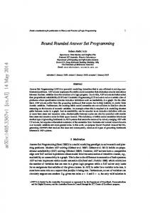
only 283 rules, the original ILASP algorithm takes 486.2s to solve the task. This is due to the scalability issues discussed in section 4 as there are 332437 violating hypotheses found before the first inductive solution. For the same task with ILASP2, there are only 9 violating reasons found before the first inductive solution, meaning that ILASP2 takes only 0.69s to solve the task. As this is the first work on learning weak constraints, there are no existing benchmarks suitable for testing our approach of learning from ordered answer sets. We have, therefore, further investigated the interview scheduling example discussed throughout the paper. Our experiments, in particular, test whether ILPLOAS can successfully learn weak constraints from examples of brave and cautious orderings. For the purpose of presentation, we assume our hypothesis space, SM , to be defined by the mode declarations: Mh = Mb = ∅; Mo = {assign(v, v), neq(v, v), type(v, c)}; Mw = {−1, 1}; and finally, lmax = 2. We place several restrictions on the search space in order to remove equivalent rules. The size of SM is 184 (our hypotheses can be any subset of these 184 rules, so even considering only hypotheses with up to 3 rules this gives over a million different hypotheses). The learning task uses background knowledge B from Example 3. As SM only contains weak constraints, for any H ⊆ SM , AS (B ∪ H ) = AS (B ). The learning tasks described in these experiments therefore correspond to learning to rank the answer sets of B . Hypothesis predictive accuracy 1
0.9
0.9
0.8
0.8 Average accuracy
Average accuracy
Hypothesis predictive accuracy 1
0.7 0.6 0.5 0.4 0.3
0.7 0.6 0.5 0.4 0.3
0.2
0.2
0.1
0.1
0
5 orderings 10 orderings 20 orderings
0 0
2
4
6
8 10 12 14 16 18 20
0 10 20 30 40 50 60 70 80 90 100
Number of examples
Fullness of examples (%)
(a)
(b)
Fig. 1: Accuracy with varying (a) numbers of examples; (b) fullness of examples For each experiment we randomly selected 100 hypotheses, each with between 1 to 3 weak constraints from SM , omitting hypotheses that ranked all answer sets equally. The only atoms that vary in B are the assign’s. As there are 9 different slots, there are 29 answer sets of B (and many more partial interpretations which are extended by these answer sets). We say an example partial interpretation is full if it specifies the truth value of all 9 assign atoms, otherwise we describe the fullness as the percentage of the 9 atoms which are specified. In both experiments (for each of the 100 target hypotheses HT ), we generated ordered pairs of partial interpretations o = he1 , e2 i such that o was bravely respected. If o was also cautiously respected, then it was given as a cautious example (otherwise it was used as a brave example). In our first experiment we investigated the effect of varying the number of examples, and in the second we investigated the effects of varying the fullness of the examples.
12
M. Law, A. Russo, K. Broda
800 600 400 200 0
4 day timetables 1200 Running time (s)
Running time (s)
1000
|SM| = 184 |SM| = 92
1000
|SM| = 184 |SM| = 92
800 600 400 200 0
0 20 40 60 80 100120 Number of examples
5 day timetables 1200 Running time (s)
3 day timetables 1200
1000
|SM| = 184 |SM| = 92
800 600 400 200 0
0 20 40 60 80 100120 Number of examples
0 20 40 60 80 100120 Number of examples
Fig. 2: Average running time of ILASP2 with varying numbers of examples In both experiments, we tested our approach 20 times for each target hypothesis HT . Each time, we used ILASP 2 to learn a hypothesis HL which covered all examples. We then calculated the accuracy of HL in predicting the pairwise ordering of answer sets in B (for each pair of answer sets A1 , A2 ∈ AS (B ) we tested whether HT and HL agreed on the preference between them). In our first experiment we investigated the effect of varying the number of examples from 0 to 20. The examples were of random fullness, each with between 5 to 9 assign atoms specified. Figure 1(a) shows the average predictive accuracy. Each point on the graph corresponds to 2000 learning tasks (100 target hypotheses with 20 different sets of examples). The error bars on the graph show the standard error. The results show that our method achieves 90% accuracy for this experiment with around 10 or more random examples. For our second experiment we again tested our approach on 100 randomly generated hypotheses with 20 different sets of randomly generated examples. This time, however, we have kept the number of examples fixed at 5, 10 and 20 and varied the fullness of the examples. Results are shown in Figure 1(b). The graph shows that examples are only useful if they are more than 50% full. One interesting point to note is that the peak performance is with examples of around 90% fullness. This is because cautious ordering examples are actually more useful if they are less full (as there are more pairs which extend them); however, orderings are less likely to be cautiously respected when they are less full. In our final experiment, we investigated the scalability of ILASP2 by increasing both the number of days in our timetable and the number of examples. Figure 2 shows the average running time for ILASP2 with 3, 4 and 5 day timetables (each with 3 slots) with up to 120 ordering examples. The learning tasks are targeted at learning the hypothesis from Example 3. We randomly generated ordering examples, as in the previous experiments with the slight difference that the fullness of the examples was unrestricted. As the hypothesis in these experiments does not use negative weights in either of the weak constraints, we also tested the average running time with a search space containing only positive weights. This means that SM contained 92 weak constraints rather than the original 184. These experiments show that the time taken to solve an ILASP2 task is dependent not only on the number of examples, but also on the size of the domain and the size of SM .
Learning Weak Constraints in Answer Set Programming
13
6 Related Work In (Law et al. 2014) we showed that any of the learning tasks in (Corapi et al. 2012; Ray 2009; Sakama and Inoue 2009; Otero 2001) could be expressed by ILPLAS and computed by ILASP. As any ILPLAS task can be (trivially) mapped into an ILPLOAS (i.e. O b = ∅ and O c = ∅), ILPLOAS inherits this property. None of the previous learning tasks (including ILPLAS ), however, can construct examples which incentivise the learning of a hypothesis containing a weak constraint. This is because they can only give examples of what should (or shouldn’t) be an answer set of B ∪ H . In addition, ILPLOAS inherits the capability of ILPLAS of supporting predicate invention, allowing new concepts to be invented whilst learning. The ILASP2 algorithm is an extension of the original ILASP algorithm in (Law et al. 2014). It extends the concepts of positive and violating hypothesis to cover learning weak constraints (which was not possible in ILASP). For the simpler ILPLAS tasks, ILASP2 is more efficient than ILASP. As discussed in section 4, the original ILASP algorithm has some scalability issues when there is a large number of violating hypotheses. We have shown in section 5 that by eliminating violating reasons rather than single violating hypotheses, ILASP2 can be much more efficient. Also related to our work are existing approaches for learning to rank. These use non logic-based machine learning techniques (e.g. neural networks (Geisler et al. 2001)). Our approach shares the same advantages as any ILP approach versus a non logicbased machine learning technique: learned hypotheses are structured, human readable and can express relational concepts such as minimising the instances of particular combinations of predicates. Existing background knowledge can be taken into account to capture predefining concepts and the search can be steered towards particular types of hypotheses using a language bias. Furthermore, ILASP2 is also capable of learning preferences with weights and priorities, meaning that more structured and complex preferences can be learned. An example of the use of an ILP system for learning constraints has been recently presented in (Lallouet et al. 2010) where timetabling constraints are learned from positive and negative examples. In this case the learned rules are hard constraints (e.g., enforcing that a teacher is not in two places at once). Examples of this kind are already computable by ILPLAS , and so are also computable by ILPLOAS . 7 Conclusion and Future Work We have presented a new framework for ILP, Learning from Ordered Answer Sets, which extends previous ILP systems in that it is able to learn weak constraints and can be used to perform preference learning. The framework can represent partial examples under a brave and a cautious semantics. We have also put forward a new algorithm, ILASP2, that can solve any ILPLOAS task for optimal solutions. This algorithm extends previous work for solving the simpler task ILPLAS and resolves some of the scalability issues associated with the previous algorithm. Some scalability issues remain, especially when there is a particularly large hypothesis space and future work will focus on overcoming these. Current work also addresses extending the ILASP algorithm to support noisy examples.
14
M. Law, A. Russo, K. Broda References
Banbara, M., Soh, T., Tamura, N., Inoue, K., and Schaub, T. 2013. Answer set programming as a modeling language for course timetabling. Theory and Practice of Logic Programming 13, 4-5, 783–798. Blockeel, H. and De Raedt, L. 1998. Top-down induction of first-order logical decision trees. Artificial intelligence 101, 1, 285–297. Calimeri, F., Faber, W., Gebser, M., Ianni, G., Kaminski, R., Krennwallner, T., Leone, N., Ricca, F., and Schaub, T. 2013. ASP-Core-2 input language format. https://www.mat.unical.it/aspcomp2013/files/ASP-CORE-2.0.pdf. Corapi, D., Russo, A., and Lupu, E. 2010. Inductive logic programming as abductive search. In ICLP (Technical Communications). 54–63. Corapi, D., Russo, A., and Lupu, E. 2012. Inductive logic programming in answer set programming. In Inductive Logic Programming. Springer, 91–97. Dastani, M., Jacobs, N., Jonker, C. M., and Treur, J. 2001. Modeling user preferences and mediating agents in electronic commerce. In Agent Mediated Electronic Commerce. Springer, 163–193. ´ ski, M. 2009. Denecker, M., Vennekens, J., Bond, S., Gebser, M., and Truszczyn The second answer set programming competition. In Logic Programming and Nonmonotonic Reasoning. Springer, 637–654. ¨ rnkranz, J. and Hu ¨ llermeier, E. 2003. Pairwise preference learning and ranking. Fu In Machine Learning: ECML 2003. Springer, 145–156. Gebser, M., Kaminski, R., Kaufmann, B., Ostrowski, M., Schaub, T., and Schneider, M. 2011. Potassco: The Potsdam answer set solving collection. AI Communications 24, 2, 107–124. Geisler, B., Ha, V., and Haddawy, P. 2001. Modeling user preferences via theory refinement. In Proceedings of the 6th international conference on Intelligent user interfaces. ACM, 87–90. ´ th, T. 2012. A model of user preference learning for content-based recommender Horva systems. Computing and informatics 28, 4, 453–481. Kimber, T., Broda, K., and Russo, A. 2009. Induction on failure: learning connected horn theories. In Logic Programming and Nonmonotonic Reasoning. Springer, 169–181. Lallouet, A., Lopez, M., Martin, L., and Vrain, C. 2010. On learning constraint problems. In Tools with Artificial Intelligence (ICTAI), 2010 22nd IEEE International Conference on. Vol. 1. IEEE, 45–52. Law, M., Russo, A., and Broda, K. 2014. Inductive learning of answer set programs. In Logics in Artificial Intelligence (JELIA 2014). Springer. Law, M., Russo, A., and Broda, K. 2015a. The ILASP system for learning answer set programs. https://www.doc.ic.ac.uk/~ ml1909/ILASP. Law, M., Russo, A., and Broda, K. 2015b. Proof of the soundness and completeness of ILASP2. https://www.doc.ic.ac.uk/~ ml1909/Proofs_for_ILASP2.pdf. Law, M., Russo, A., and Broda, K. 2015c. Simplified reduct for choice rules in ASP. Tech. Rep. DTR2015-2, Imperial College of Science, Technology and Medicine, Department of Computing. Muggleton, S. 1991. Inductive logic programming. New generation computing 8, 4, 295–318. Muggleton, S., De Raedt, L., Poole, D., Bratko, I., Flach, P., Inoue, K., and Srinivasan, A. 2012. ILP turns 20. Machine Learning 86, 1, 3–23. Muggleton, S. and Lin, D. 2013. Meta-interpretive learning of higher-order dyadic datalog: Predicate invention revisited. In Proceedings of the Twenty-Third international joint conference on Artificial Intelligence. AAAI Press, 1551–1557.
Learning Weak Constraints in Answer Set Programming
15
Otero, R. P. 2001. Induction of stable models. In Inductive Logic Programming. Springer, 193–205. Ray, O. 2009. Nonmonotonic abductive inductive learning. Journal of Applied Logic 7, 3, 329–340. Ray, O., Broda, K., and Russo, A. 2004. A hybrid abductive inductive proof procedure. Logic Journal of IGPL 12, 5, 371–397. Sakama, C. and Inoue, K. 2009. Brave induction: a logical framework for learning from incomplete information. Machine Learning 76, 1, 3–35. Srinivasan, A. 2001. The aleph manual. Machine Learning at the Computing Laboratory, Oxford University.
16
M. Law, A. Russo, K. Broda Appendix A The ILASP2 Meta Encoding
We present here the ILASP2 meta encoding which is omitted from the main paper. We first summarise some notation used in the encoding. We will write body + (R) and body − (R) to refer to the positive and negative (respectively) literals in the body of a rule R. Given a program P , weak (P ) denotes the weak constraints in P and non weak (P ) denotes the set of rules in P which are not weak constraints. Definition 8 For any ASP program P , predicate name pred and term term we will write reify(P , pred , term) to mean the program constructed by replacing every atom a ∈ P by pred(a, term). We will use the same notation for sets of literals/partial interpretations, so for a set S : reify(S , pred , term) = {pred(atom, term) : atom ∈ S }. Definition 9 For any ASP program P and any atom a, append (P , a) is the program constructed by appending a to every rule in P . Definition 10 Given any term t and any positive example e, cover (e, t ) is the program: inc exc exc cov(t):-in as(einc 1 , t), . . . , in as(en , t), not in as(e1 , t), . . . , not in as(em , t). :-not cov(t).
The previous three definitions can be used in combination to test whether a program has an answer sets which extend given partial interpretations. Example 5 Consider the program P =
�
p:-not q. q:-not p.
�
and the partial interpretations I1 =
h{p}, ∅i and I2 = h∅, {p}i. The program Q = append (reify(P , in as, X ), as(X )) ∪ {as(as1), as(as2)} ∪ cover (I1 , as1) ∪ cover (I2 , as2) has the grounding: in_as(p, in_as(q, in_as(p, in_as(q,
as1) as1) as2) as2)
::::-
not not not not
in_as(q, in_as(p, in_as(q, in_as(p,
as1), as1), as2), as2),
as(as1). as(as1). as(as2). as(as2).
as(as1). as(as2). cov(as1) :- in_as(p, as1). :- not cov(as1). cov(as2) :- not in_as(p, as2). :- not cov(as2).
Without the two constraints, Q would have 4 answer sets (the combinations of as1 and as2 corresponding to the two answer sets of P ). With the two constraints,
17
Learning Weak Constraints in Answer Set Programming
the answer set represented by as1 must extend I1 , and the answer set represented by as2 must extend I2 . Hence, there is only one answer set of Q , {as(as1), as(as2), in as(p, as1), in as(q, as2), cov(as1), cov(as2)}. Note that the answer sets of P which extend I1 and I2 ({p} and {q}) can be extracted from the in as atoms in this answer set of Q . If there were multiple answer sets of P extending one or more of the partial interpretations, then there would be multiple answer sets, representing all possible combinations such that the constraints are met. Definition 11 Let p1 and p2 be distinct predicate names and t be a term. Given R, a weak constraint :∼ b1 , . . . , bm , not c1 , . . . , not cl .[wt@lev, t1 , . . . , tn ], metaweak (R, p1 , p2 , t ) is the rule: w(wt, lev, args(t1 , . . . , tn ), t):-p2 (X), p1 (b1 , t), . . . , p1 (bm , t),not p1 (c1 , t), . . . , not p1 (cl , t).
For a set of weak constraints W , metaweak (W , p1 , p2 , t ) is the set {metaweak (R, p1 , p2 , t ) | R ∈ W }. Example 6 Consider the program P containing the two weak constraints: :~ p(V).[1@2, V] :~ q(V).[2@1, V]
metaweak (P , in as, as, X ) is the program: w(1, 2, args(V), X) :- as(X), in_as(p(V), X). w(2, 1, args(V), X) :- as(X), in_as(q(V), X).
Note that for any program P , if we reify an interpretation I = {a1 , . . . , an } as {in as(a1 , id), . . . , in as(an , id)} (the set reify(I , in as, id )) then the atoms w(wt, l, args(t1 , . . . , tm ), id) in the (unique) answer set of metaweak (weak (P ), in as, as, X ) ∪ reify(I , in as, id ) ∪ {as(id)} correspond exactly to the elements (wt , l , t1 , . . . tm ) of weak (P , I ). For example, consider the interpretation I = {p(1), p(2), q(1)}. The unique answer set of metaweak (weak (P ), in as, as, X )∪reify(I , in as, id )∪{as(id) } is {as(id), in as(p(1), id), in as(p(2), id), in as(q(1), id), w(1, 2, args(1), id), w(1, 2, args(2), id), w(2, 1, args(1), id)}. In this case, weak (P , I ) = {(1, 2, 1), (1, 2, 2), (2, 1, 1)}. Now that we have defined the predicate w to represent weak (P , A) for each answer set A, we can use some additional rules to determine, given two interpretations, whether one dominates another. Definition 12 Given any two terms t 1 and t 2, dominates(t 1, t 2) is the program: dom lv(t1, t2, L):-lv(L), #sum{w(W, L, A, t1) = W, w(W, L, A, t2) = −W} < 0.
non dom lv(t1, t2, L):-lv(L), #sum{w(W, L, A, t2) = W, w(W, L, A, t1) = −W} < 0. non bef(t1, t2, L):-lv(L), lv(L2), L < L2, non dom lv(t1, t2, L2). dom(t1, t2):-dom lv(t1, t2, L), not non bef(t1, t2, L).
18
M. Law, A. Russo, K. Broda
The intuition is that dom(id1, id2) (where id1 and id2 represent two answer sets A1 and A2 ) should be true if and only if A1 dominates A2 . This is dependent on the atoms dom lv(id1, id2, l), which for each level l , should be true if and only if PAl 1 < PAl 2 ; non dom lv(id1, id2, l), which for each level l , should be true if and only if PAl 2 < PAl 1 ; and finally, non bef(id1, id2, l), which for each level l , should be true if and only if there is an l2 > l such that PAl22 < PAl21 . Example 7 Consider again the program P and interpretation I from example 6. Consider also an additional interpretation I ′ = {p(1), p(2), p(3)}. weak (P , I ′ ) = {(1, 2, 1), (1, 2, 2), (1, 2, 3)}. The unique answer set of metaweak (weak (P ), in as, as, X ) ∪ reify(I , in as, id 1) ∪ reify(I ′ , in as, id 2) ∪ {as(id1), as(id2), lv(1), lv(2)} ∪ dominates(id 1, id 2) contains dom lv(id1, id2, 2), because I dominates I ′ at level 2 (i.e. PI2 < PI2′ ); contains non dom lv(id1, id2, 1), because I ′ dominates I at level 1; does not contain any non bef atoms, because the only level at which I ′ dominates I is 1, which is not evaluated “before” any other level (it is the lowest level in the program); and finally, does contain dom(id1, id2) because I dominates I ′ at level 2 and there is no level “before” (higher than) level 2 at which I ′ dominates I . The presence of dom(id1, id2) in the answer set indicates that I dominates I ′ . Similarly, the unique answer set of metaweak (weak (P ), in as, as, X ) ∪ reify(I , in as, id 1) ∪ reify(I ′ , in as, id 2) ∪ {as(id1), as(id2), lv(1), lv(2)} ∪ dominates(id 2, id 1) contains dom lv(id2, id1, 1), because I ′ dominates I at level 1; contains non dom lv(id2, id1, 2), because I dominates I ′ at level 2; contains non bef(id2, id1, 1) as I dominates I ′ at level 2, which is evaluated “before” level 1; and finally, does not contain dom(id2, id1) because there is no level l in the program such that I ′ dominates I at l and I does not dominate I ′ at any higher level. A.1 Encoding the search for positive hypotheses: Tmeta We now use the components described in the previous section to define a program Tmeta whose answer sets correspond to the positive solutions of an ILPLOAS task T. Definition 13 Let T be the ILPLOAS task hB , SM , E + , E − , O b , O c i. Then Tmeta = meta(B ) ∪ meta(SM ) ∪ meta(E + ) ∪ meta(E − ) ∪ meta(O b ) ∪ meta(O c ) where each meta component is as follows: • meta(B ) = append (reify(non weak (B ), in as, X ), as(X )) ∪ metaweak (weak (B ), in as, as, X ). • meta(SM ) = {append (append (reify(R, in as, X ), as(X )), in h(Rid )) | R ∈ non weak (SM )} ∪ {append (W , in h(Wid )) | W ∈ metaweak (weak (SM ), in as, as, X )} ∪ {:∼ in h(Rid ).[2 ∗ |R|@0, Rid ] | R ∈ SM } ∪ { {in h(Rid ) : R ∈ SM }. }
Learning Weak Constraints in Answer Set Programming � � cover (e, eid ) inc exc + + • meta(E ) = he , e i ∈ E as(eid ). inc n), . . . , in as(einc n , n), v i:-in as(e1 ,exc inc exc not in as(e1 , n), . . . , − − he , e i ∈ E • meta(E ) = not in as(eexc m , n). as(n). � � violating:-v i. ∪
19
:∼ not violating.[1@0]
as(oid1 ). as(oid2 ). cover (e 1 , oid1 ) • meta(O b ) = cover (e 2 , oid2 ) dominates(oid1 , oid2 )
o = he1 , e2 i ∈ O b ∪{lv(l). | l ∈ L} :-not dom(oid1 , oid2 ). � � dominates(e1 , e2 ) v p:-v p(T1, T2). 1 2 c c • meta(O ) = v p(eid , eid ): he1 , e2 i ∈ O ∪ violating:-v p. not dom(e1 , e2 ).
The intuition is that the in h atoms correspond to the rules in the hypothesis. Each rule R ∈ SM has a unique identifier Rid and if in h(Rid ) is true then R is considered to be part of the hypothesis H . These in h atoms have been added to the bodies of the rules in the meta encoding so that a rule R ∈ SM only has an effect if it is part of H . Each of the terms t for which there is a fact as(t) represents an answer set of B ∪ H . As in the previous section the cover program cover (I , t ) is used to enforce that some of these answer sets extend particular partial interpretations. There is one as(t) atom for each positive example e. The cover program is used to ensure that the corresponding answer set does extend e. There are two as(t) atoms for each brave ordering he1 , e2 i. Two instances of the cover program are used to ensure that the first answer set extends e1 and the second answer set extends e2 . We also use the dominates program from the previous section and a constraint to ensure that the first answer set dominates the second (hence the ordering is bravely respected). For the negative examples and the cautious orderings, the aim is to generate violating in at least one answer set of the meta encoding corresponding to H , if H is indeed a violating solution (generating v i if H does not cover a negative example and some instance of v p if it does not respect a cautious ordering). Firstly, for the negative examples, we have an extra fact as(n). As we have no constraints on the answer set of B ∪ H which this can correspond to, the intuition is that there is one answer set of the meta encoding for each answer set of B ∪ H . For each negative example e − there is a rule for v i which will generate v i if the answer set corresponding to as(n) extends e − . For the cautious orderings we use a similar approach. For any cautious ordering he1 , e2 i, as e1 and e2 are positive examples, there are already two as(t) atoms which represent answer sets extending each of these interpretations; in fact, there will be one answer set of the meta encoding for each possible pair of answer sets of B ∪ H
20
M. Law, A. Russo, K. Broda
which extend these interpretations. Therefore, by using the dominates program, and generating a v p atom if the answer set of B ∪ H corresponding to the first as(t) atom does not dominate the answer set of B ∪ H corresponding to the second as(t) atom in any answer set of the meta encoding, we ensure that violating will be true in at least one answer set of the meta encoding which corresponds to H . Example 8 Consider the learning task: p(V):-r(V), not q(V). q(V):-r(V), not p(V). r(1). r(2). B= a:-not b. b:-not a. q(1). SM = :∼ q(V).[1@1, V, r2]
h{p(2)}, ∅i, h∅, {p(2)}i, + E = h{a}, {b}i, h∅, {a}i � E − = � h{p(1)}, ∅i O b = � he3+ , e4+ i O c = he1+ , e2+ i
:∼ b.[1@1, b, r3]
Figure A 1 shows Tmeta . There are two optimal positive hypotheses (one containing each of the two weak constraints). The positive hypothesis :∼ b · [1@1, b, r3] has a violating interpretation {p(1), q(2), r(1), r(2), a}. This corresponds to the following answer set of Tmeta : { as(1), as(2), as(3), as(4), as(n), as(5), as(6), lv(1), in_as(r(1),1), in_as(r(1),2), in_as(r(1),3), in_as(r(1),4), in_as(r(1),n), in_as(r(1),5), in_as(r(1),6), in_as(r(2),1), in_as(r(2),2), in_as(r(2),3), in_as(r(2),4), in_as(r(2),n), in_as(r(2),5), in_as(r(2),6), in_as(q(1),3), in_as(q(1),4), in_as(q(1),6), in_as(p(1),1), in_as(p(1),2), in_as(p(1),n), in_as(p(1),5), in_as(p(2),1), in_as(q(2),2), in_as(q(2),3), in_as(q(2),4), in_as(q(2),n), in_as(q(2),5), in_as(q(2),6), in_as(a,1), in_as(a,2), in_as(a,3), in_as(b,4), in_as(a,n), in_as(a,5), in_as(b,6), in_h(r2), w(1,1,args(2,r2),2), w(1,1,args(1,r2),3), w(1,1,args(2,r2),3), w(1,1,args(1,r2),4), w(1,1,args(2,r2),4), w(1,1,args(2,r2),n), w(1,1,args(2,r2),5), w(1,1,args(1,r2),6), w(1,1,args(2,r2),6), cov(1), cov(2), cov(3), cov(4), v_i, violating, dom_lv(1,2,1), dom(1,2), cov(5), cov(6), dom_lv(5,6,1), dom(5,6) }
Note that the violating interpretation can be extracted from the in as( , n) atoms and the hypothesis can be extracted from the in h atoms. Similarly, the violating pair h{p(2), q(1), r(1), r(2), a}, {p(1), q(2), r(1), r(2), a}i can be extracted from the answer set: { as(1), as(2), as(3), as(4), as(n), as(5), as(6), lv(1), in_as(r(1),1), in_as(r(1),2), in_as(r(1),3), in_as(r(1),4), in_as(r(1),n), in_as(r(1),5), in_as(r(1),6), in_as(r(2),1), in_as(r(2),2), in_as(r(2),3), in_as(r(2),4), in_as(r(2),n), in_as(r(2),5), in_as(r(2),6), in_as(q(1),1), in_as(q(1),4), in_as(q(1),6), in_as(p(1),2), in_as(p(1),3), in_as(p(1),n), in_as(p(1),5), in_as(p(2),1), in_as(q(2),2), in_as(q(2),3), in_as(q(2),4), in_as(q(2),n), in_as(q(2),5), in_as(q(2),6), in_as(a,1), in_as(a,2), in_as(a,3), in_as(b,4), in_as(a,n), in_as(a,5), in_as(b,6), w(1,1,args(1,r2),1),
Learning Weak Constraints in Answer Set Programming
21
in_h(r2), w(1,1,args(2,r2),2), w(1,1,args(2,r2),3), w(1,1,args(1,r2),4), w(1,1,args(2,r2),4), w(1,1,args(2,r2),n), w(1,1,args(2,r2),5), w(1,1,args(1,r2),6), w(1,1,args(2,r2),6), cov(1), cov(2), cov(3), cov(4), v_i, violating, v_p(1,2), v_p, cov(5), cov(6), dom_lv(5,6,1), dom(5,6) }
% meta(B) in_as(p(V),X) :- in_as(r(V),X), not in_as(q(V),X), as(X). in_as(q(V),X) :- in_as(r(V),X), not in_as(p(V),X), as(X). in_as(r(1),X) :- as(X). in_as(r(2),X) :- as(X). in_as(a,X) :- not in_as(b,X), as(X). in_as(b,X) :- not in_as(a,X), as(X). % meta(S_M) in_as(q(1),X) :- as(X), in_h(r1). w(1,1,args(V,r2),X) :- in_as(q(V),X), as(X), in_h(r2). w(1,1,args(b,r3),X) :- in_as(b,X), as(X), in_h(r3). 0 {in_h(r1), in_h(r2), in_h(r3)} 2. :~ in_h(r1).[2@0,r1] :~ in_h(r2).[2@0,r2] :~ in_h(r3).[2@0,r3] % meta(E^+) as(1). as(2). as(3). as(4). cov(1) :- in_as(p(2),1). cov(2) :- not in_as(p(2),2). cov(3) :- in_as(a,3), not in_as(b,3). cov(4) :- not in_as(a,4). :- not cov(1). :- not cov(2). :- not cov(3). :- not cov(4).
% meta(E^-) v_i :- in_as(p(1),n). as(n). violating :- v_i. :~ not violating.[1@0, violating] % meta(O^b) as(5). as(6). cov(5) :- in_as(a,5), not in_as(b,5). cov(6) :- not in_as(a,6). :- not cov(5). :- not cov(6). dom_lv(5,6,L) :- lv(L), #sum{w(W,L,A,5)=W, w(W,L,A,6)=-W} < 0. wrong_dom_lv(5,6,L) :- lv(L), #sum{w(W,L,A,6)=W, w(W,L,A,5)=-W} < 0. wrong_bef(5,6,L) :- lv(L), L < L2, wrong_dom_lv(5,6,L2). dom(5,6) :- dom_lv(5,6,L), not wrong_bef(5,6,L). :- not dom(5,6). lv(1). % meta(O^c) dom_lv(1,2,L) :- lv(L), #sum{w(W,L,A,1)=W, w(W,L,A,2)=-W} < 0. wrong_dom_lv(1,2,L) :- lv(L), #sum{w(W,L,A,2)=W, w(W,L,A,1)=-W} < 0. wrong_bef(1,2,L) :- lv(L), L < L2, wrong_dom_lv(1,2,L2). dom(1,2) :- dom_lv(1,2,L), not wrong_bef(1,2,L). v_p(1,2) :- not dom(1,2). v_p :- v_p(X,Y). violating :- v_p.
Fig. A 1: An example of Tmeta .
22
M. Law, A. Russo, K. Broda A.2 Encoding classes of violating hypotheses: VRmeta
The previous section set out how to construct a meta level ASP program Tmeta whose answer sets correspond to the positive hypotheses. It is also able to identify violating hypotheses, but has no way of eliminating them (as only a subset of the meta level answer sets corresponding to a violating hypothesis will identify it as violating, so eliminating these answer sets does not necessarily eliminate the hypothesis). We therefore present a new meta level program which, combined with Tmeta , eliminates any hypothesis which is violating for a given set of violating reasons. As violating reasons are full answer sets (or pair of full answer sets), we do not have to generate answer sets. It is enough to check whether the answer sets we have as part of the violating reasons are still answer sets of B ∪ H . The standard way to do this is check whether these answer sets are the minimal model of the reduct of B ∪ H with respect to this answer set. The next two definitions define a meta level program which, given an interpretation, computes the minimal model of the reduct of a program with respect to that interpretation. This reduct construction is close to the simplified reduct for choice rules from (Law et al. 2015c). Definition 14 Given any choice rule R = l{h1 , . . . , hn }u:-body, reductify(R) is the program: + − mmr(h1 , X):-reify(body , mmr, X), reify(body , not in vs, X), l{in vs(h1 , X), . . . , in vs(hn , X)}u, in vs(h1 , X)· ... + − mmr(hn , X):-reify(body , mmr, X), reify(body , not in vs, X), l{in vs(h1 , X), . . . , in vs(hn , X)}u, in vs(hn , X)·
mmr(⊥, X):-reify(body+ , mmr, X), reify(body− , not in vs, X), vs(h u + 1{in 1 , X), . . . , in vs(hn , X)}· + − mmr(⊥, X):-reify(body , mmr, X), reify(body , not in vs, X), {in vs(h1 , X), . . . , in vs(hn , X)}l − 1·
Definition 15 Let P be an ASP program such that P1 is the set of normal rules in P , P2 is the set of constraints rules in P . � in P and P3 is the set of choice � mmr(head(R), X):-reify(body+ (R), mmr, X), reductify(P ) = R ∈ P1 reify(body− (R), not in vs, X), vs(X). � � mmr(⊥, X):-reify(body+ (R), mmr, X), R ∈ P2 ∪ − reify(body (R), not in vs, X), vs(X).
∪ {reductify(R) | R ∈ P3 }·
Example 9 � � p:-not q. Consider the program P = q:-not p. � � mmr(p, X):-not in vs(q, X), vs(X). reductify(P ) = mmr(q, X):-not in vs(p, X), vs(X).
We can check whether {p} is an answer set by combining reductify(P ) with
Learning Weak Constraints in Answer Set Programming
23
{vs(vs1), in vs(p, vs1)}. The answer set of this program is {vs(vs1), in vs(p, vs1), mmr(p, vs1)}, from which the minimal model, {p}, can be extracted. This shows that {p} is indeed an answer set of P . Definition 16 Let T be the ILPLOAS task hB , SM , E + , E − , O b , O c i and VR be the set of violating reasons VI ∪VP , where VI are violating interpretations and VP are violating pairs. VRmeta (T ) is the program meta(VI ) ∪ meta(VP ) ∪ meta(Aux ) where the meta components are defined as follows: reify(I , in vs, Iid ) I ∈ VI • meta(VI ) = :-not nas(Iid ). vs(Iid ). dominates(vpid1 , vpid2 ) reify(I , in vs, vp ) id1 1 reify(I , in vs, vp ) 2 id2 • meta(VP ) = vs(vpid1 ). vp = hI1 , I2 i ∈ VP vs(vpid2 ). :not nas(vp id1 ), not nas(vpid2 ), not dom(vpid1 , vpid2 ).
• meta(Aux ) = reductify(B ) � � nas(X):-in vs(ATOM, X), not mmr(ATOM, X). ∪ nas(X):-not in vs(ATOM, X), mmr(ATOM, X). ∪ {append (reductify(R), in hyp(Rid )) | R ∈ non weak (SM )} ∪ {append (metaweak (W , in vs, vs, X ), in hyp(Wid )) | W ∈ weak (SM )} ∪ {metaweak (W , in vs, vs, X ) | W ∈ weak (B )} ∪ {lv(l). | l ∈ L}
This meta encoding uses the reductify program to check whether the various interpretations in each violating reason is still an answer set of B ∪ H . There is a constraint for each of the violating interpretation, ensuring that it is no longer an answer set of B ∪H . Similarly, there is a constraint for each violating pair that says, if both interpretations are still answer sets of B ∪ H , then the first must dominate the second. This is checked by using the dominates program as before (the weak constraints are also translated as before). Example 10 Recall B , SM , E + , E − , O b and O c from example 8 and let VI be the set containing the violating interpretation {p(1), p(2), r(1), r(2), a}, VP the set containing the violating pair h{p(2), q(1), r(1), r(2), a}, {q(1), q(2), r(1), r(2), a}i and let VR be the set of violating reasons VI ∪ VP . Then figure A 2 shows VRmeta (T ). Now that we have ruled out any hypothesis with these violating reasons, one optimal answer set of this program is:
{ as(1), as(2), as(3), as(4), as(n), as(5), as(6), lv(1), in_vs(p(1),v1), in_vs(p(2),v1), in_vs(r(1),v1), in_vs(r(2),v1), in_vs(a,v1), vs(v1), in_vs(p(2),v2), in_vs(q(1),v2), in_vs(r(1),v2), in_vs(r(2),v2), in_vs(a,v2),
24
M. Law, A. Russo, K. Broda
vs(v2), in_vs(q(1),v3), in_vs(q(2),v3), in_vs(r(1),v3), in_vs(r(2),v3), in_vs(a,v3), vs(v3), in_as(r(1),1), in_as(r(1),2), in_as(r(1),3), in_as(r(1),4), in_as(r(1),n), in_as(r(1),5), in_as(r(1),6), in_as(r(2),1), in_as(r(2),2), in_as(r(2),3), in_as(r(2),4), in_as(r(2),n), in_as(r(2),5), in_as(r(2),6), in_as(q(1),1), in_h(r1), in_as(q(1),2), in_as(q(1),3), in_as(q(1),4), in_as(q(1),n), in_as(q(1),5), in_as(q(1),6), in_as(p(2),1), in_as(q(2),2), in_as(p(2),3), in_as(q(2),4), in_as(p(2),n), in_as(p(2),5), in_as(q(2),6), in_as(a,1), in_as(a,2), in_as(a,3), in_as(b,4), in_as(a,n), in_as(a,5) in_as(b,6), w(1,1,args(1,r2),1), in_h(r2), w(1,1,args(1,r2),2), w(1,1,args(2,r2),2), w(1,1,args(1,r2),3), w(1,1,args(1,r2),4), w(1,1,args(2,r2),4), w(1,1,args(1,r2),n), w(1,1,args(1,r2),5), w(1,1,args(1,r2),6), w(1,1,args(2,r2),6), cov(1), cov(2), cov(3), cov(4), w(1,1,ts(1),v2), w(1,1,ts(1),v3), w(1,1,ts(2),v3), dom_lv(1,2,1), dom(1,2), cov(5), cov(6), dom_lv(5,6,1), dom(5,6), mmr(r(1),v1), mmr(r(1),v2), mmr(r(1),v3), mmr(r(2),v1), mmr(r(2),v2), mmr(r(2),v3), mmr(p(1),v1), mmr(p(2),v1), mmr(p(2),v2), mmr(q(1),v2), mmr(q(1),v3), mmr(q(2),v3), mmr(a,v1), mmr(a,v2), mmr(a,v3), mmr(q(1),v1), nas(v1), dom_lv(v2,v3,1), dom(v2,v3) }
This answer set corresponds to the hypothesis: q(1). :~ q(V).[1@1,V,r2]
As the optimality of this answer set is 5, we know that this hypothesis cannot have any violating reasons, as otherwise, there would be an answer set with optimality 4 corresponding to the hypothesis (which would have been returned as optimal). Hence, the hypothesis must be an optimal inductive solution of the task.
Learning Weak Constraints in Answer Set Programming
25
#sum{w(W,L,A,v3)=W, w(W,L,A,v2)=-W} < 0. wrong_bef(v2,v3,L) :- lv(L), L < L2, wrong_dom_lv(1,2,L2). dom(v2,v3) :- dom_lv(v2,v3,L), not wrong_bef(v2,v3,L).
% meta(VI) in_vs(p(1),v1). in_vs(p(2),v1). in_vs(r(1),v1). in_vs(r(2),v1). in_vs(a,v1). vs(v1). :- not nas(v1).
:- not nas(v2), not nas(v3), not dom(v2,v3).
% meta(VP) in_vs(p(2),v2). in_vs(q(1),v2). in_vs(r(1),v2). in_vs(r(2),v2). in_vs(a,v2). vs(v2).
% meta(Aux) mmr(p(V),X) :- mmr(r(V),X), not in_vs(q(V),X), vs(X). mmr(q(V),X) :- mmr(r(V),X), not in_vs(p(V),X), vs(X). mmr(r(1),X) :- vs(X). mmr(r(2),X) :- vs(X). mmr(a,X) :- not in_vs(b,X), vs(X). mmr(b,X) :- not in_vs(a,X), vs(X).
in_vs(q(1),v3). in_vs(q(2),v3). in_vs(r(1),v3). in_vs(r(2),v3). in_vs(a,v3). vs(v3). dom_lv(v2,v3,L) :- lv(L), #sum{w(W,L,A,v2)=W, w(W,L,A,v3)=-W} < 0. wrong_dom_lv(v2,v3,L) :- lv(L),
mmr(q(1),X) :- vs(X), in_h(r1). w(1,1,ts(V),X) :- vs(X), in_vs(q(V),X), in_h(r2). w(1,1,args(b,r3),X) :- vs(X), in_vs(b,X), in_h(r3). nas(X) :- in_vs(A,X), not mmr(A,X). nas(X) :- not in_vs(A,X), mmr(A,X).
Fig. A 2: An example of VRmeta (T ).