LECTURE NOTE NAME OF COURSE: FLUID MECHANICS II ...

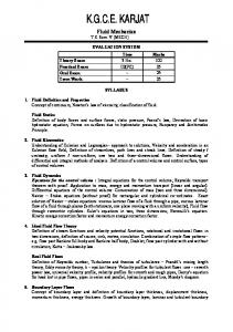
LECTURE NOTE

NAME OF COURSE:

FLUID MECHANICS II

COURSE CODE:

MCE 305

UNITS:

3

LECTURER:

KUYE, S. I.

INTRODUCTION The air we breathe, the water we drink, and the blood and other liquids that flow in our bodies demonstrate the close dependence of our lives on various fluids. Not only must these fluids, as well as many others, be present when we need them, it is important that they are present where we need them with not only satisfactory quality; but also sufficient quantity.

NATURE AND TYPE OF FLUID Nature of Fluid What is a fluid? A fluid is a substance that deforms continuously under the action of a shear force. A fluid may be a liquid or a gas; it offers resistance to a change of shape and is capable of flowing. Liquid and gas are distinguished as follows: •

A gas completely fills the space in which it is contained; a liquid usually has a free surface.

•

A gas is a fluid which can be compressed relatively easily and is often treated as such; a liquid can be compressed only with difficulty.

TYPE OF FLUID Fluids can be classified according to their behaviours under stress as Newtonian fluids or non-Newtonian fluids.

Newtonian Fluids These are fluids which obey Newton’s law viscosity which says the shear stress is linearly related to the rate of shear strain or velocity gradient. Most common fluids such as water, gasoline, ethanol, fall into this category.

Non-Newtonian Fluids These are fluids which do not obey Newton’s law of viscosity. The group includes: (i) Plastic - the shear stress must a reach a certain (minimum) value before flow Commences. Thereafter, shear stress increases with the rate of shear according to the relationship

τ = A + B du dy   

n

(1.1)

Where A and B are constants. if n = 1 ,

τ = A + B du dy  



This is called Bingham plastic

(ii) Pseudoplastic The dynamic viscosity, µ of the fluid decreases as the rate of shear increases (e.g. milk, clay, colloidal solutions, sewage, sludge, cement). If n < 1 in Eq.(1.1), it is called pseudoplastic.

(iii) Dilatant Substances The dynamic viscosity,

µ

increases as the rate of shear increases e.g.

quicksand. If n > 1 in Eq.(1.1), it is called dilatant.

(iv) Thioxotropic Substances The dynamic viscosity decreases with the time for which shearing forces are applied e.g. thioxotropic jelly paints.

(v) Rheopectic Materials The dynamic viscosity of these materials increases with the time for which shearing forces are applied.

(vi) Viscoelastic Materials These behave in manner similar to Newtonian fluids under time-invariant conditions but if shear stress changes suddenly behave as plastic.

THE FLUID AS A CONTINUUM A continuum is a phase or a continuous distribution of matter with no voids. A fluid is said to be a continuum because the formulation of the basic relationships is based

on a hypothetical continuous fluid; a fluid that can be continually subdivided without thought of a molecular structure. This approach avoids the difficulty of dealing with the complexity of molecular motion itself. Although, certain fluid properties are explained on the basis of molecular considerations.

PHYSICAL PROPERTIES OF FLUID These are those characteristics common to all fluids which are directly of interest to engineers. The properties to be considered here are •

Density

•

Specific weight

•

Relative density or specific gravity

•

Viscosity

•

Surface tension

•

Compressibilty

•

Pressure

SCOPE OF FLUID MECHANICS Fluid mechanics is the science that deals with fluids at rest and in motion.

In this study of fluid mechanics we shall be concerned with fundamental principle which will help us better in understanding the behaviours of fluids.

UNITS AND CONSTRAINTS

FLUID STATICS This is the concept of fluid at rest. Studying the behaviour of fluids at rest is of prime importance to the engineer. Generally, fluids exert both normal and shearing forces on surfaces that are in contact with them. However, only fluids with velocity gradients produce shearing forces. A static fluid will exert a normal force on any boundary that it is in contact with. These boundaries may be large and the force may differ from place to place, hence it is convenient to work in terms of pressure, p.

Pressure

It is defined as the force per unit area. It is basically a surface force exerted by a fluid against the walls of its containing vessel. •

Pascal established that the pressure at any point within a stationary fluid is the same in all directions and it is dependent of its orientation.

•

For a static fluid, pressure varies only with elevation within the fluid.

Pressure Measurement There are so many pressure measuring devices, they include barometer, piezometer, Bourdon gauge and manometer

A barometer is used to measure the atmospheric pressure in absolute units, it is one of the few “absolute” pressure gauges.

By measuring the liquid level or levels in columns of tubes connected to a tank in which the pressure is to be measured and applying the hydrostatic equations, manometers can be used to obtain the desired pressures. Different types of manometers are
Piezometer; the simplest form of manometer
U-tube manometer
U-tube with one leg enlarged
Inverted U-tube manometer
Differential manometer Limitations of Manometer as Pressure Gauge  Manometer cannot be used conveniently for large pressure differences.  Some liquids do not form well-defined menisci, therefore unsuitable  Effect of surface tension is unavoidable due to capillary rise. Although this can be avoided if the diameter of the tubes are sufficiently large (< 15mm diameter)  It is unsuitable for measuring fluctuating pressures because of its slow response

 Inaccurate readings are obtainable due to slight fluctuations of pressure which causes the liquid in the manometer to oscillate. However, these oscillations can be minimised by putting restrictions in the manometer connections  At times, air bubbles are entrapped within the tubes. But to avoid this, the pipes connecting the manometer to the pipe or vessel containing the liquid under pressure should be filled with this liquid and that there should be no air bubbles in the liquid.

EQUILIBRIUM OF FLUID AT REST

THRUST ON PLANE SURFACES

BUOYANCY Whenever a body is immersed wholly or partially in a fluid it is subjected to an upward force which tends to lift it up. This tendency for an immersed body to be lifted up in fluid, due to an upward force opposite to action of gravity is known as buoyancy. The force tending to lift up the body under such conditions is known as buoyant force or force of buoyancy or upthrust. The magnitude of the buoyant force can be determined by Archimedes’ principle which states that “when a body is immersed in a fluid either wholly or partially, it is buoyed or lifted up by a force, which is equal to the weight of fluid displaced by the body”.

THRUSTS ON CURVED SURFACES

INTEGRAL ANALYSIS Control Volume (CV) This is a designated region in space through which a particular amount of fluid passes. Its size and shape may be arbitrarily selected to suit the requirements of the problem, but must then be held constant.

The bounding surface of the control volume is termed the control surface, CS. Generally equation that describe the motion of the fluid as it passes through the CV is Eulerian.

Reynold’s Transport Theorem The use of control volume does not permit a direct application of physical laws as known from mechanics. Since the 2nd law of Newton relates the force to the rate of change of momentum of a body of matter, i.e. , a control mass, the rate of change of momentum of a body contained in a CV is not directly and simply related to the forces acting on it.

Reynold’s transport theorem provides the necessary relationship between the control mass and control volume approach. It is given by

dN ∂ r r = ∫cvηρdV + ∫csηρu .dA dt ∂t

3.1

where, η =specific property

dV =differential volumetric element r dA =outward area vector r u =velocity in the sense of the flow direction In effect, Reynold’s transport theorem states that the rate at which the property

N increases with time within the system is equal to the time rate of increase of N in the CV plus the net rate of flow of N through the CS.

Mass Conservation The principle of mass conservation stipulates that the mass of a system remains constant. But the mass contained within a CV may not be constant since the fluid moves across the bounding surface, the CS. For obtaining the rate of change of mass contained within the CV, Reynold’s transport equation (3.1) is used with η = 1(for mass, η =

mass = 1 ) to obtain mass

dm ∂ r r = ∫cv ρdV + ∫cs ρu .dA dt ∂t

3.2

where, m is the mass contained within the CV at time t. For mass conservation

dm =0 dt ∂ r r ρ dV + ρ u ∫ ∫cs .dA ∂t cv ∂ r r i.e. ρ dV = − ρ u ∫ ∫cs .dA ∂t cv so, 0 =

3.3

This equation holds for any CV and states that the rate of accumulation of mass within a CV equals the net rate of flow of mass through the CS.

Continuity Equation in One- Dimensional Flow This is usually developed from the general principle of the law of conservation of mass which states that the mass within a system remains constant with time i.e.

dm = 0 . If M is the mass contained in the CV at time t, from equation (3.3) dt ∂ r r ρ dV + ρ u ∫ ∫cs .dA = 0 ∂t cv Assuming the flow to be steady, the first term drops out, hence

r r

∫cs ρu.dA = 0

3.4

Eq. (3.4) must be applied to each CS where fluid mass is entering or leaving; therefore

∫

r

r

cs1

r

r

ρ1u1 .dA1 + ∫cs ρ 2u 2 .dA2 = 0

3.5

2

If the inlet and outlet velocity vectors are, at each inlet and outlet, perpendicular to their respective areas, then all outflow integral dot products are evaluated as

r

r

ρ 2 u 2 .dA2 = ρ 2 u 2 dA2

3.6

and inflow are

r

r

ρ1u1 .dA1 = − ρ1u1dA1 So,

If

3.7

∫ ρ u dA = ∫ ρ u dA cs1

1 1

1

cs2

2

2

2

ρ1 and ρ 2 do not vary across the inlet and outlet areas, then

3.8

ρ1 ∫cs u1 dA1 = ρ 2 ∫cs u 2 dA2 1

3.9

2

If u1 A1 = ∫cs u1 dA1 , u 2 A2 = ∫cs u 2 dA2 1

2

then Eq. (3.9) becomes

ρ1u1 A1 = ρ 2 u 2 A2 = m&

3.10

If the discharge Q is defined as

Q = Au the continuity equation may take the form

m& = ρ1Q1 = ρ 2 Q2 For incompressible steady flow

Q = A1u1 = A2 u 2 is a useful form of the equation for constant density flow, steady or unsteady

r r u ∫cs .dA = 0

3.11

which states that the net volume efflux is zero. This implies that the CV is filled with liquid at all times. The, since there is no flow across the wall of the stream tube, Eq. (3.10) is the continuity equation applied to two sections along a stream tube in a steady flow for a “compressible” flow. For incompressible flow, Eq. (3.11) can be written properly as

u1 A1 = u 2 A2 = Q

3.12

FLUID IN MOTION The science of a fluid in motion is most conveniently studied using energy methods. The fluid will be assumed to be an incompressible fluid (liquid).

BERNOULLIS THEOREM Energy of a Flowing Fluid Potential energy: This is due to its elevation above datum. If a weight W of liquid is at a height z above datum. Potential energy (P.E.) = WZ So, potential energy/unit weight =

Wz =z W

This is referred to as potential head.

Pressure energy: When a fluid flows in a continuous stream under pressure it can do work. If the area of cross-section of the stream of fluid is A then force due to pressure p on cross-section is pA . If a weight W of liquid passes the cross-section the volume passing cross-section =

W

γ

Distance moved by liquid =

W γA

Work done = Force x Distance = pA ×

Pressure energy per unit weight =

p

γ

W pW p = = W = pressure energy γA γ γ

= pressure head

Note: pressure energy is the energy of a liquid flowing under pressure.

Kinetic energy: If a weight W of liquid has a velocity v, kinetic energy =

W 2 v where, W = mg 2g

v2 kinetic energy per unit weight = = velocity head 2g v2 The total energy per unit weight = z + + γ 2g p

Total head = potential head + pressure head + velocity head

v2 H =z+ + γ 2g p

3.13

Eq. 3.13 is useful in the analysis of a fluid flow system by considering two points at a time along the system. If suffices 1, 2 denote two points A, B, respectively, in a pipe according to the figure shown below, then for a liquid flowing in the pipe from A to B,

p1

2

2

v p v + 1 + z1 = 2 + 2 + z 2 = constant γ 2g γ 2g

Eq. (3.14) is known as Bernoullis equation.

3.14

Bernoullis theorem states that the total energy of each particle of a body of fluid is the same provided that no energy enters or leaves the system at any point. The derivation and application of Eq. 3.14 has been based on the following assumptions (i) Incompressible fluid (ii) No mechanical devices (pumps, turbines) (iii)No heat transfer (iv) No friction

ELEMENTARY CONSIDERATION OF VISCOUS FLUID

DIMENSIONAL ANALYSIS This is the reorganization of the dimensional variables important to a particular problem so as to obtain a lesser number of dimensionless parameters. It is a useful technique for the investigation of problems in all branches of engineering particularly in fluid mechanics.

The starting point is the logical premise that a relationship describing a physical phenomenon operating under natural laws must be dimensionally homogeneous. That is, every term in the relationship must have identical dimensions. Such a relationship is written as an equation which describes how the dependent variable varies with the independent variables. These relationships can be established by two classes of methods. (i) Developing a mathematical model of the phenomenon. In this case the operating physical laws are expressed in the form of equations. Almost always some assumptions have to be made that simplify the situation to a point at which the resulting mathematics can be performed. Such a simplified mathematical model may represent the situation quite accurately but sometimes the simplifying assumptions are so drastic that the model bears a little relation to the physical problem. (ii) Construction of a physical model. This method is used when the mathematical approach does not give good results, or the problem is complicated that no mathematical model can be developed no matter the assumptions made, sometimes such problems involve so many variables. Measurements of

parameters of interest can be taken from this model and scaling laws are then used to derive values applicable to the real situation (the prototype).

Dimensions All variables can be derived from quite a small number of certain basic entities. These are called dimensions, for example, length, breadth and height. They are measured properties used to describe the physical state of the body or system. In describing dimensions, agreeable units of measurement are used. The fundamental quantities and their S. I. units and symbols are given below.

Quantity

Units

Dimension

Length

Metres

L

Mass

Kilogramme

M

Time

Second

T

Force

Newton

F

Temperature

Kelvin

O

When the thermodynamic effects are not required, the four dimensions of length, mass, time and force are sufficient to describe mechanics behaviour. The four dimensions do not exist independently but are related through Newton’s second law. The dimensions of all other variables can be expressed in terms of these fundamental dimensions. For instance velocity has the dimension of L/T as it is the ratio of distance travelled to the time taken.

THE BUCKINGHAM PI-THEOREM First theorem A relationship between a set of physical variables can be stated as a relationship between a set of independent dimensionless groups made up from suitably chosen variables.

Second theorem The number of dimensionless groups required to specify completely the relationship is the number of variables, n, minus the number of dimensions, m, involved in the variables. These dimensionless groups are often called pi groups.

Grouping of typical variables: (i) Geometric variable: (ii) Flow variables Kinematic: Dynamic: (iii) Fluid properties:

The first group is the geometric variables, generally length dimensions are used. Alternatively, the cross-sectional area or on occasion, even a volume could be used. The second group consists of kinematic and dynamic variables: velocity, discharge, time and acceleration are the most common kinematic variables. The dynamic variable include the shearing stress, pressure difference, pressure gradient, force, and power. The final group contains the fluid properties.

Repeating variables These are variables that repeat themselves in the pi groups of a problem. The number is equal to m (the fundamental dimensions in the problem).

The guidelines for picking the repeating variables are listed in ni particular order below: 1. All the fundamental dimensions occurring in the problem must be found in at least one of the m repeating variabvles. 2. Pick variables that appear to be important over the range of operating conditions. 3. No two repeating variables should have identical dimensions. 4. Chose one repeating variable from each of the three groups. If m = 2 , variables may be chosen from only two of the groups. 5. Select repeating variables from the independent variables.

MODELLING Modelling is a particular type of experimental behaviour embarked upon in design before the construction of a prototype. In modern day engineering practice, any new type of machine or structure involving interaction with fluids is seldom constructed

until a model test has been made. Scale models are model systems proportioned after the original systems such that the quantitative physical behaviour of the original system or the prototype can be inferred from the observed quantitative behaviour of the model, even though the model may have smaller

SIMILARITY Similarity is a term found when it comes to model testing, and its laws are very necessary when it comes to translating a model into a prototype. There are two types of similarity; Geometric similarity and dynamic similarity.

Geometric Similarity This deals with the geometry of the model and the prototype. In this sense, it means that the model should be an exact geometric replica of the prototype. Geometric similarity is only achieved in model testing but the case becomes invalid when it comes to situations like river models where distortion of the vertical scale is necessary to obtain meaningful results.

Dynamic Similarity In dynamic similarity, the forces which act on corresponding masses in the model and prototype should be in the same ratio throughout the area of flow modelled in fluid flow. If this similarity is achieved, it follows that the flow pattern will be identical for both the model and the prototype flow fields.

TYPICAL NON-DIMENSIONAL PARAMETERS Some dimensionless terms have been, by convention and convenience, assigned particular names. These are as follows

∆p = Eu (Euler number) ρv 2 / 2 The factor of 2 is added arbitrarily to make the denominator equal to the dynamic pressure of the flow.

v = Fr (Froude number) Dγ / ρ In most cases it can be simplified to

v Dg

Fr =

Also

vDρ

µ

=

vD

ν

= Re (Reynolds number)

v = We (Weber number) σ / ρD It can also be written as

ρDv 2 We = σ v = Ma (Mach or Cauchy number) E/ρ or Ma =

ρv 2 E

FLOW IN PIPES Most theoretical investigations in nthe field of fluid dynamics are based on the concept of a perfect, i.e. frictionless and incompressible fluid. In the motion of such a perfect fluid, two contacting layers experience no tangential forces but act on each other with normal forces (pressures) only.

However, the inner layers of a real fluid transmit tangential as well as normal stresses, this being also the case near a solid wall wetted by a fluid. These tangential or friction forces in a real fluid are connected with a property which is called the viscosity of the fluid.

Recall Newton’s law of viscosity

τ ∞ dv dy This makes us to understand that the shear stress in a fluid is proportional to the velocity gradient, which is the rate of change of velocity across the fluid path. For Newtonian fluids we have

τ = − µ dv dy Flow of fluids is usually described in terms of flow regimes namely laminar and turbulent flow regimes. Between the two ends is the transition zone.

Laminar and turbulent flow Consider a pipe through which there is flow of water, into which a dye has been injected. Three situations are possible on the flow path that is described by the dye.
It is possible that the dye is observed to flow in a straight path.
Another possibility is that, the dye describes a path that looks like a wave front that is characterized by hills and valleys.
The third and last possibility is that an increased level of disoderliness will be observed on the flow path of the dye in the flowing water stream.

While the first situation occurs when the main fluid stream is flowing slowly, the last one occurs when it is flowing fast.

The straight path case represents laminar flow while the irregular flow path of random disorderliness represents turbulent flow. Fluid flow in pipes is basically a function of four variables namely: fluid density (), flow velocity (v), pipe diameter (D) and fluid dynamic viscosity (). For circular pipes, these variables are put together in a dimensionless quantity known as Reynolds number, which is written as

Re, N R or N R e. By definition

Re =

Inertial force on fluid element Viscous force on fluid element

From Newton’s second law, inertial force is defined as

Fi = ma And the viscous force is given as

Fv = τ A In terms of the four variables given above

Re =

uDρ

µ

The kinematic viscosity

ν = µρ Re =

i.e.

uD

ν

it can be interpreted that when the inertial forces dominate over the viscous forces (when the fluid is flowing faster and Re is large) then the flow is said to be turbulent, when the viscous forces are dominant (slow flow, low Re), they are sufficient enough to keep all the fluid particles in line, then the flow is laminar. The following features characterize the flow regimes.

Laminar flow o Re < 2000 o Low velocity o Fluid particles move in straight lines o Rare in practice

Turbulent flow o Re > 4000 o High velocity o Fluid particles path is completely irregular o Average motion is in the direction of flow o Most common type of flow

Energy Equation The energy equation is a more general flow equation than the Bernoullis’ equation as it accounts for energy addition and energy loss during fluid flow. Recall that Bernoullis’ equation is based on the following assumptions: -

Fluid is incompressible

-

No pumps/turbines are installed on the flow path

-

No friction/energy losses

-

No heat transfer

Though, heat transfer is typically negligible, in the real sense of it, no system has all the restrictions listed in the Bernoullis equation. Three energy terms in addition to the pressure, velocity and elevation heads are included in the energy equation. These are

hA = Energy added to the system by mechanical device (pump) hR =Energy removed (motor/turbine) hA = Energy losses (friction + minor losses) The magnitude of friction head loss is proportional to the velocity head.

 v2  hL = k    2g  where k is known as resistance coefficient.

ENTRY CONDITIONS THE BOUNDARY LAYER CONCEPT When a fluid flows over a stationary surface such as the wall of a pipe, the part touching the surface is brought to rest by the shear stress at the wall. The velocity of the fluid increases from the wall to a maximum in the main stream of the flow, as illustrated below. max

v=0 wall

This profile does not just exist, it must build up gradually from the point where the fluid starts to flow past the surface, when it enters a pipe for example.

If we consider a flat plate in the middle of a fluid, we will look at the build up of the velocity profile as the fluid moves over the plate. Upstream, the velocity is uniform, a long way downstream we have the velocity profile that is illustrated above. This region where there is a velocity profile in the flow due to the shear stress at the wall is called the boundary layer. Boundary layer grows from zero when the fluid starts to flow over a solid surface. As it passes over a greater length, more fluid is slowed by friction between the fluid layers close to the boundary, hence the thickness of the slower layer increases. The

fluid near the top of the boundary layer is dragging the fluid nearer to the solid surface along, by one of two mechanisms. The first type occurs when the normal viscous forces are large enough to exert drag effects on the slower moving fluid close to the solid boundary. If the boundary layer is thin then the velocity gradient normal to the surface, du

dy

is large. By Newton’s law of viscosity τ = µ

du dy

is also large.

The corresponding force may then be large enough to exert drag on the fluid close to the surface.

As the boundary layer thickness becomes greater, so the velocity gradient becomes smaller and the shear stress decreases until it is no longer enough to drag the slow fluid near the surface along. If this viscous force was the only action, then the fluid would come to a rest. It , does not come to a rest but the second mechanism comes into play.

PRESSURE LOSSES IN BENDS AND PIPE FITTINGS Since turbulent flow is the condition most common in engineering systems, the head loss for a fitting is usually specified as a fraction of the kinetic energy head,

 v2  hL = C L    2g  The non-dimensional factor C L is termed as the loss coefficient and, in general, depends on the geometry of the fitting and the Reynold’s number. For practical flow calculations, however, it is conventional to use the highest value of C L independent of

Re D , giving slightly conservative results. Table below gives the representative values of these loss coefficients for some standard pipe fittings.

Fitting

CL

Fitting

Elbows (bends)

CL

Globe valve

45o

0.4

fully open

90o

0.9

half open

180o

0.9

10 20

Unions Tee

Gate valve

Along run

0.4

fully open

0.3

Along branch

1.0

half open

5

Loss coefficients of some standard fittings

SUDDEN CHANGE OF SECTION Head losses at sudden area changes are associated with trapped eddies which are formed when the boundary layer separates in the region of increasing pressure. There can be abrupt expansion or abrupt contraction.

D2 V1

D1

V1

D2

V2

D1

V2

1 2

1

2

(a) Abrupt expansion

(b) Abrupt contraction

PIPE FITTINGS AND VALVES

DIFFUSERS The head loss at an abrupt enlargement (or the exit from a pipe) can be considerably reduced by the substitution of a gradual, tapered, enlargement usually known as a diffuser or recuperator. Its function is to reduce the velocity of the fluid gradually and thus eliminate, as far as possible, the eddies responsible for the dissipation of energy. Eddies occur at a discontinuity in the pipe surface, such as a sudden enlargement or contraction. At a discontinuity of section or obstruction the boundary layer breaks away from the pipe surface to form the eddy.

NOZZLES, BRANCHED PIPES AND FLOW DISTRIBUTION SYSTEMS

FLOW MEASUREMENTS DEVICES Venturi meter

h flow V1

V2

B A

C

Fig. A venturi meter

The flow rate of liquid in a closed pipe is measured by a venture meter. This consists of a constriction in the pipe line as shown. The pipe converges in the direction of flow from the flange A to the throat B, and then diverges gradually to the full pipe diameter at C. Manometer tubes inserted in the pipe at A and at the throat B enable the pressure difference between the two points to be measured. The flow rate of

liquid in the pipe is then proportional to the square root of the pressure difference or manometric head h .

Orifice Liquid under a static head h is allowed to flow through an orifice, whose diameter is small compared with the head as shown in the figure. The velocity v of the issuing jet is then obtained by equating the pressure energy or head of the liquid in the tank to its kinetic energy or velocity head at the jet. Neglecting energy losses, the theoretical velocity of flow v is given by

h=

v2 or v = 2 gh 2g

h y

Fig. An orifice

Weirs Open-channel flow may be measured by a weir, which is an obstruction in the channel that causes the liquid to back up behind it and flow over it or through it. The rate of flow is determined by measuring the height of upstream liquid surface. L y

x H

δy

H L

ϕ