Light confinement and propagation characteristics in plasmonic gap waveguides on silicon Rafael Salas-Montiela , Sylvain Blaizea , Aur´elien Bruyanta , Aniello Apuzzoa , Gilles Lerondela , C´ecile Delacourb , Philippe Grosseb , Jean-Marc Fedelib and Alexei Tchelnokovb a Laboratoire
de Nanotechnologie et d’Instrumentation Optique, UTT, Troyes 10010, France; b CEA LETI, DOPT 17 rue des Martyrs, Grenoble 38054, France ABSTRACT
Plasmonic waveguiding structures have the ability to confine and propagate light over short distances, typically less than a hundred micrometers. This short propagation length is the price that is paid for confining light to dimensions on the order of a hundred of nanometers. With these scales in mind, several plasmonic devices can be proposed (e.g. wavelength multiplexors) and some of them have been already demonstrated such as Y junctions and directional couplers. Although the dimensions involved in such structures are below the diffraction limit, large-scale optical characterization techniques, such as transmitted power, are still employed. In this contribution, we present a characterization technique for the study of the guided modes in plasmonic gap waveguiding structures that resolves subwavelength-scale features, as it is based on atomic force microscope and on near field scattering optical microscope in guided detection with a lateral resolution of about λ/9. Keywords: surface plasmonic gap waveguides, silicon waveguides, near field scattering optical microscopy, optical directional couplers, integrated plasmonic devices
1. INTRODUCTION Metal gap waveguides are one of the most studied plasmonic waveguides, mainly because such structures provide the best trade-off between propagation loss and confinement of plasmon waves.1 Typically, the confinement scale in such structures is well below the diffraction limit, and the propagation length is in tens of micrometers. Therefore, metal gap structures could lead to compact, highly integrated photonic devices.2 Efforts have been made to fabricate silicon-gold couplers using planar technology to efficiently couple optical power carried by an optical mode from a silicon-on-insulator (SOI) waveguides into plasmonic gap waveguides.3–5 As current optical tests (i.e. optical power transmission) can not resolve subwavelength-scale dimensions, complementary characterization techniques are needed. Near-field scanning optical microscopy (NSOM) provides a remarkable access to the waveguiding properties in plasmonic structures. Between aperture and apertureless NSOM configurations for the study of optical waveguiding structures, the apertureless NSOM has been privileged mainly because it can be implemented from existing atomic force microscopy (AFM). In addition, current AFM probes feature a typical tip radius of less than 10 nm, giving the required resolution for the investigation of photonic structures. Transmission-based apertureless NSOM has successfully been applied for the characterization of glass6 and lithium niobate waveguides,7 as well as on silicon-based structures.8 This technique, which was proposed in Ref.,9 measures the change in transmission at the device output induced by the AFM probe. Our motivation here is to demonstrate that the NSOM in a guided detection configuration is a simple yet powerful technique for probing plasmonic devices. In order to do so, we have characterized a vertically coupled copper plasmon gap waveguide on silicon fabricated with conventional planar microelectronic technology. We will show the optical NSOM images acquired by the use of this technique, and we will interpret them by a simple interference model between the plasmon mode and the scattered field induced by the sample-tip interaction. Finally, we will compare the experimental results to finite difference time domain (FDTD) numerical simulations of the vertically integrated coupler on Si. Further author information: (Send correspondence to R.S.M.) R.S.M.: E-mail: rafael.salas
[email protected], Telephone: +33(0)325718001 S.B.: E-mail:
[email protected], Telephone: +33 (0)325xxxxxx
2. EXPERIMENTAL 2.1 Description and fabrication process development A detailed description of the coupler and its principle of operation can be found in.10 Here, we present a brief description of the coupler and its fabrication process. The structure is a vertically integrated directional coupler with Si and Cu waveguides fabricated with standard Si technology at the CEA-Leti. We have represented the coupler schematically in Fig. 1.
Figure 1: Vertically coupled Cu gap waveguide on Si. As a starting material we used a standard SOI wafer in which the 220-nm-thick Si layer lays on top a 2µm buried oxide layer. Deep UV lithography was used to pattern the Si layer and reactive ion etching (RIE) was then used to form the Si waveguide. The width of the Si waveguide was fixed to 400 nm for a singlemode operation at a wavelength of 1550 nm. A gap of 6µm in the Si waveguide has been done to ensure that the transmitted optical power is not propagating through the Si waveguide. To facilitate the coupling with optical fibers, tapers at the input and at the output of the waveguide have been added with a final width of 2µm. Afterwards, the waveguide was embedded in a 320-nm-thick SiO2 layer and planarized with chemical mechanical polishing (CMP). Two coplanar trenches were then photolithographically defined, partially RIE etched (70 nm), and filled with a 50-nm-thick Cu layer. Finally, the Cu in excess was removed with CMP. At the coupling zone, the vertical separation of the waveguides is 30 nm.
2.2 Setup for the measurement of the optical near field Experimental data were obtained by probing the optical near field of the light propagating through the coupling device with an AFM-based NSOM in guided detection. The setup is an arrangement of a conventional integrated optics setup and a commercial AFM probe.
Figure 2: Optical near field setup. A tunable laser source is used to couple light into the device with a tapered lens single-mode polarization maintaining fiber. A fiber polarization controller, a Polarization Beam Splitter (PBS), and a half-wave retarder are employed to fix a state of polarization at the device input. The polarized signal (quasi-TE or quasi-TM) is then butt-coupled into the device, and the transmitted power density is detected using a second tapered lens SMF connected to a lock-in amplifier via an InGaAs detector. A dielectric AFM probe, set to intermittent contact mode at frequency f0 , is then used to locally perturb the optical near field of the mode. As a result, the photodetector measures an a.c. electrical signal of frequency f0 . The lock-in amplifier amplifies the signal and then multiplies it by the lock-in reference. The product of this multiplication yields a d.c. output signal
proportional to the component of the signal whose frequency is exactly locked to the reference frequency. The low pass filter, which follows the multiplier, removes the components at all other frequencies increasing the signal-to-noise ratio. The lock-in amplifier can be then locked to either f0 , 2f0 , or 3f0 to single out the first, second, and third components and therefore accurately measure the optical near field. At the same time, an image representing the surface topology is obtained by monitoring the changes in the oscillation amplitude of the probe. As the AFM probe scans the surface of the waveguide in a intermittent contact mode, the evanescent field of the guided light is scattered away from the surface. Let us see the Fig. 3 to understand the physical working principle of the NSOM in a guided detection configuration.
Figure 3: Physical working principle of the NSOM in a guided detection. ~ in the electric field injected in the waveguiding structure and we do not take into account any If we call E possible reflected electric fields, we can confirm that the electric field after the interaction with the AFM tip is ~ 2 = t1 (z0 ) · k(nf0 )E ~ in , where t1 (z0 ) is the transmission coefficient and k(nf ) is the scattering coefficient that E ~ out , which is the electric field describes the interaction sample-to-tip. If we consider the relationship between E ~ 2 , i.e E ~ out = t2 (z0 − L) · E ~ 2 , we can write E ~ out = t1 (z0 ) · k(nf0 ) · t2 (z0 − L)E ~ in at the end of the structure, and E 2 or, in others words, Pout = T1 T2 |K(nf0 )| Pin . In the last equation T1 and T2 are the intensity transmission coefficients at the input and at the output air-silicon interface ports, Pin is the input optical power, and |K(f0 )|2 is the square magnitude response of the probe-to-sample interaction. During the probe scan, the optical power immediately beyond the probe is P2 = P1 − Psca , where P1 is the optical power carried by the guided mode and Psca is the power scattered by the probe. Consequently the square magnitude response |K(nf0 )|2 is thus P2 /P1 = 1 − Psca /P1 and the overall intensity transmission change measured at the detector is: ZZ h i 1 ~ sca × H ~ ∗ ·n ~ dS E sca Psca 2 , ∆T = = Z ZS h (1) i 1 P1 ~1×H ~ ∗ · ~z dA E 1 2 A∞
~ is a unitary vector orthogonal to S, A∞ is the waveguide cross where S is a surface enclosing the probe, n section, and ~z is the unitary vector along the direction of propagation. Here, we assumed that the waveguide is singlemode at the incident wavelength and that it is invariant along the direction of propagation. Moreover, ~ sca (~r ) and the under the hypothesis of a vertical confined field and a passive probe, the relation between the E ′ 11 ~ local electric field is E sca (~r ): Z ~ sca (~r) = ~ sca (~r ′ )dV ′ , E G(~r , ~r′ ) · ∆ǫ · E (2) V
where G denotes the Green function in the free space in the far-field approximation, ∆ǫ = ǫprobe − ǫCu , and V is the volume enclosing the probe. As a a consequence of eq. (2) that one of the most crucial problems about the interpretation of NSOM measurements lies in modeling the shape of the tip (i.e the volume V) and its optical properties (i.e the quantity ǫprobe ) as described in detail in the section 3.4. We deduce that the time dependence ~ sca follows as exp(jωt + φ) exp[−jγZ(t)], where φ(~r ) is the local phase of the optical guided field over the of E waveguide surface at the scanner position defined by the Cartesian coordinates (~r , Z = 0), γ is the decay length
along the Z axis, and Z(t) = A + A cos(2πf0 t) is the signal applied to the probe12 with an amplitude A. To conclude, a more appropriate mathematical approach for the interpretation of the results of the optical near field measurements is the signal processing approach.13 This consists in writing the transfer function of each path segment. However, this will be the topic of another study based on the transfer matrix S1 , ST , S2 .
3. RESULTS In this section, we display and analyze the experimental results obtained with the use of the setup for the measurement of the optical near field. The plasmonic device is as described in the Fig. 1 for working wavelength of 1550 nm. In addition, we analyze the modal and the propagation characteristics of the surface plasmonic gap waveguide numerically. Indeed, the mode profiles and effective indices for this structure can not be solved analytically, therefore we have calculated them with the finite element method and with the finite difference time domain method implemented in the commercial software FEMsim and Fullwave both by Rsoft. Femsim was used as a mode solver to calculate the mode distributions in the Si and Cu waveguides. The calculated mode profiles and effective indices for the Si waveguide were used then as excitation inputs for the simulation of the coupler with the use of fullwave. In all simulation we use 1.445 and 0.46743 + j0.445 as indices of refraction for the SiO2 and the Cu both at a wavelength of 1550nm.
3.1 Experimental results As is known, the lateral resolution of an AFM image is determined by its step size and the radius of the probe. Considering that the size of the smallest images we took were 10 µm by 10 µm with 512 by 512 data points, the step size is 20 nm. The 30 µm by 30µm images in Fig. 4 are the first result we measured.
Figure 4: Superposition of two AFM and two NSOM optical images of the plasmonic coupleur. From the AFM images, the length of the plasmonic gap waveguide is 7.45 µm and the average height is 20 ± 5 nm. The gap width is 190 nm and the metal width is 520 nm. In the NSOM image, the incident field from the input SOI waveguide is at the left side. In Fig. 5 we can see a single 30 µm by 30µm image of the mode propagation through the plasmonic gap waveguide.
Figure 5: AFM and NSOM optical images of the vertically integrated plasmonic gap waveguide on Si. The insertion loss, defined as the ratio of the output to the input optical powers, can be estimated from this result. Indeed, the optical power is the integral of the power density profile over a cross section of the SOI waveguides. Accordingly, the insertion loss is 2.2 ± 0.1 dB at a wavelength of 1550 nm. A detailed image of the NSOM signal is shown in Fig. 6 where the second harmonic of detection (i.e. 2f0 ) was selected. A standing wave pattern, with a period Λ, can be observed as a result of the interference between the coand counter-propagative gap modes. We have plotted as well the average cross-section profiles of the gap mode
15
15
−1500
1500
−2000 −2500 10
10
1000
y (µm)
y (µm)
−3000 −3500 −4000
500
5
5 −4500 −5000 0
0 0
−5500 5
10
0 0
15
5
x (µm)
10
15
x (µm)
(a) AFM image.
(b) NSOM image at 2f0 .
Figure 6: Measured gap mode propagation. for the first, second, and third lock-in amplifier harmonics to observe the influence of the detection at different demodulation references.
|E|2 (a.u.)
1
f0 2f0 3f0 fdtd sim exp fit
resolution λ/9
0.5
0 -1
-0.5
0
0.5
1
x (µm)
Figure 7: Cross-section power density profiles. As shown in the Fig. 7, the evanescent fields fits to exponential functions with decay lengths of 255 nm, 210 nm, and 170 nm for n = 1, 2, and 3 respectively. An exponential function is plotted only for the third harmonic. As expected, higher harmonics allows us to measure in more detail the NSOM signal.
3.2 Mode solver calculations The real part of the effective index and the power propagation length as a function of the gap are plotted in the Fig. 8. Here, the power propagation length is defined as the length over which the optical power carried by the mode decays to e−1 its initial value and it is given by Lprop = λ0 /4πℑ{neff }. As we can see, the fundamental gap mode does not experience a cutoff width over this width range. The real part of the effective index decreases with wider gap widths and therefore becomes less confined within the gap reaching the effective index of a single Cu stripe. On the contrary, the power propagation length increases as the gap increases reaching again that of a single Cu stripe indicating that the two waves at each metal-insulator surface become decoupled. The field component distributions for the fundamental mode with a gap width of 190 nm is plotted in Fig. 9 as well as the power flow along the direction of propagation. The x-component of the electric field is well confined inside the gap with maxima power densities located at the bottom corners. For the y-component, it is clear that there is no power density at the middle of the gap because the power density is confined near the four corners of the gap again with maxima at the bottom
femsim simulations
1.9
13
Power propagation length (µm)
Real part of the effective index
1.95
1.85 1.8 1.75 1.7 1.65 1.6 1.55
Femsim
12 11 10 9 8 7 6 5 4
1.5
3 0
0.1 0.2 0.3 0.4 0.5 0.6 0.7 0.8 0.9
0
0.1 0.2 0.3 0.4 0.5 0.6 0.7 0.8 0.9
gap (µm)
gap (µm)
(a)
(b)
Figure 8: Real part of the effective index and power propagation length as a function of the gap width.
2
0.4
0
1
−0.2
1.5
0.2 y (µm)
y (µm)
0.4
1.5
0.2
1 0 0.5
−0.2
0.5
−0.4
−0.4 −1
−0.5
0 x (µm)
0.5
−1
1
−0.5
(a) |Ex |2
0.5
1
(b) |Ey |2
0.4
0.4
0.3 0.2
0
0.15 0.1
−0.2
y (µm)
0.25
0.2 y (µm)
0 x (µm)
1
0.2
0.8
0
0.6 0.4
−0.2
0.2
0.05 −0.4
−0.4 −1
−0.5
0 x (µm)
(c) |Ez |2
0.5
1
−1
−0.5
0
0.5
1
x (µm)
(d) Sz
Figure 9: Calculated gap mode profiles and z-component of the Poynting Vector.
corners. As for the z-component, the power density is the lowest of all the field components. The power flow in the direction of propagation is at the four corners of the gap and near the vertical sidewalls.
3.3 FDTD simulations The simulated total electric field and its x- and y-components as a function of space at a fixed value of time are plotted in Fig. 10.
(a) |E|2
(b) |Ex |2
(c) |Ey |2
(d) Phase of the x-component of the electric field
(e) |Ex |2 in the yz plane
Figure 10: Calculated gap mode profiles and z-component of the Poynting Vector. As we can observe, the E-field power density (Fig. 10a) is highly confined to the gap and guided along the direction of propagation z and its strength decreases as the propagation length increases. A standing wave pattern can be seen as a result of the interference between the forward and backward gap modes. For analysis, the x- and y-components are plotted as well (Fig. 10b and 10c). The behavior of these two components calculated by the FDTD method confirms the one calculated by FEM method in subsection 3.2. The phase of the x component of the electric field is plotted in Fig. 10d. The first observation to make is that, along a cross section, the phase is constant inside the dielectric gap whereas it is variable in the metal with a 180◦ change at the metal-dielectric interfaces. This changing phase is due to the spatial oscillations as the profile was calculated as a function of space at fixed value of time. Because the spatial phase is changing away int the Cu, the plasmon must be radiating in the direction away from the interface into the metal. The vertical coupling from the SOI waveguide to the Cu gap waveguide is clearly seen in Fig. 10e. As we can see in Fig. 7, the calculated profile roughly matches the measured profile. Differences can be explained first by notice that the Si and Cu waveguides are not singlemode at 1550 nm. Indeed, from the NSOM images we observe the intensity maxima shifting back and forth laterally as the modes propagate through the waveguides with different effective indices. According to modal calculations, the Si waveguide supports two modes, the quasi-TE00 and the quasi-TM00 . By using these two modes as input fields in the FDTD simulation of the all structure, we observe this mode beating throughout the Cu waveguide. The result is an asymmetrical gap mode profile matching the shape and the contrast of the measured profile as can be seen in Fig. 11 where the normalized power for the quasi-TE00 mode was 0.8 and 0.2 for the for the quasi-TM00 . Although this multimode behavior explains the shape of the profile it does not explains the gap mode profile widening. Globally, the experimental results shows a standing wave pattern that can be explained as a result of the interference between the co- and counter-propagative plasmonic gap modes. From there, the real part of the effective index of the fundamental mode is neff = λ/2Λ, where Λ is the spatial period. We measured neff = 1.64 ± 0.06 which is consistent with the calculated value of neff = 1.5832 + j0.01506 using FemSIM. A coupling
TE00 /TM00 80/20 3f0
|E|2 (a.u.)
1
0.5
0
-1
-0.5
0
0.5
1
x (µm)
Figure 11: Measured and calculated profiles with input modes as: quasi-TE00 (80%) and quasi-TM00 (20%). efficiency can be roughly estimated from the measured insertion loss of 2.2 dB at 1550 nm by considering that it consist of coupling and propagation losses. However, to determine coupling and propagation losses accurately, vertically coupled plasmonic gap waveguides with different lengths need to be fabricated and tested. Compare to free space AFM-based NSOM typical detection, the guided detection configuration increase the signal-to-noise ratio as the measured optical power is confined within the waveguiding structure and the optical fibers. The use of a digital lock-in amplifier not only allow us to amplify the optical signal but also to observe it at different reference harmonics (nf0 ) and therefore measure with high resolution the optical near field. Given that the numerical simulations were done without any scatterer placed close to the plasmonic gap waveguide (i.e. the AFM probe), the calculated mode is more confined within the gap explaining the size mismatch. Therefore, a scattering problem including the actual geometry of the probe need to be investigated with the use of eq.(2). In other words, either the probe geometry needs to be carefully modeled or the plasmonic structure that we are simulating is not accurate enough to match the measured profile. Indeed, a copper oxide layer is likely to be formed over the copper gap waveguide thus decreasing the mode confinement.
3.4 Scattering problem The probe has been modeled first by one column of N dipoles (i.e. cylindrical shape) and then by an inverted pyramidal shape. The profile of the scattered field by a cylindrical and pyramidal -shaped probe are plotted in Fig. 12. Cylindrical probe Pyramidal probe 3f0
|E|2 (a.u.)
1
0.5
0
-1
-0.5
0
0.5
1
x (µm)
Figure 12: Calculated scattered field by an AFM probe constructed of individual dipoles above the gap waveguide and measured NSOM signal. The diameter of the each dipole is 10 nm and the ambient is air. The external field, which is the gap mode profile, was calculated at a distance y = 15 nm above the surface of the waveguide. The calculated shape of the E-field scattered by a pyramidal-shaped probe matches the shape of the measured power density profile of the plasmon gap mode.
4. CONCLUSION To summarize, a vertically integrated plasmonic gap waveguide on Si has been characterized by an AFM-based near field scattering optical microscope in guided detection. The setup for the measurement of the optical near
field and a sample-to-tip model have been described. After image processing, some fundamental characteristics of the plasmonic gap waveguide were obtained. In conclusion, the NSOM technique in guided detection is a configuration with great potential for the optical characterization of planar plasmonic couplers and plasmonic devices. Subwavelength-scale dimensions with high detection and high resolution can be obtained. Combining traditional optical tests (i.e. transmission fiberdevice-fiber) with this technique provides a unique way to better understand the waveguiding properties in planar plasmonic couplers recently proposed.
REFERENCES 1. L. Chen, J. Shakya, and M. Lipson, “Subwavelength confinement in an integrated metal slot waveguide on silicon,” Opt. Lett. 31, pp. 2133–2135, 2006. 2. G. Veronis and S. Fan, “Guided subwavelength plasmonic mode supported by a slot in a thin metal film,” Opt. Lett. 30, pp. 3359–3361, 2005. 3. J. Tian, S. Yu, W. Yan, and M. Qiu, “Broadband high-efficiency surface-plasmon-polariton coupler with silicon-metal interface,” Appl. Phys. Lett. 95, 2009. 4. Z. Han, A. Y. Elezzabi, and V. Van, “Experimental realization of subwavelength plasmonic slot waveguides on a silicon platform,” Opt. Lett. 35, pp. 502–504, 2010. 5. R. Yang, R. A. Wahsheh, Z. Lu, and M. A. G. Abushagur, “Efficient light coupling between dielectric slot waveguide and plasmonic slot waveguide,” Opt. Lett. 35, pp. 649–651, 2010. 6. F. Gesuele, C. Pang, G. Leblond, S. Blaize, A. Bruyant, P. Royer, R. Deturche, P. Maddalena, and G. Lerondel, “Towards routine near-field optical characterization of silicon-based photonic structures: An optical mode analysis in integrated waveguides by transmission afm-based snom,” Physica E: Low-dimensional Systems and Nanostructures 41(6), pp. 1130 – 1134, 2009. Proceedings of the E-MRS 2008 Symposium C: Frontiers in Silicon-Based Photonics. 7. S. Tascu, P. Moretti, S. Kostritskii, and B. Jacquier, “Optical near-field measurements of guided modes in various processed LiNbO3 and LiTaO3 channel waveguides,” Optical Materials 24, pp. 297–302, 2003. 8. W. C. L. Hopman, R. Stoffer, and R. M. de Ridder, “High-resolution measurement of resonant wave patterns by perturbing the evanescent field using a nanosized probe in a transmission scanning near-field optical microscopy configuration,” J. Lightwave Technol. 27, pp. 1811–1818, 2007. 9. J. T. Robinson, S. F. Preble, and M. Lipson, “Imaging highly confined modes in sub-micron scale silicon waveguides using transmission-based near-field scanning optical microscopy,” Opt. Express 14, 2006. 10. C. Delacour, S. Blaize, P. Grosse, J. M. Fedeli, A. Bruyant, R. Salas-Montiel, G. Lerondel, and A. Chelnokov, “Efficient directional coupling between silicon and copper plasmonic nanoslot waveguides: toward metaloxide-silicon nanophotonics,” Nano Letters 10, pp. 2922–2926, July 2010. 11. C. Girard and A. Dereux, “Near-field opticas theories,” Rep. Prog. Phys. 59, pp. 657–699, 1996. 12. I. Stefanon, S. Blaize, A. Bruyant, S. Aubert, G. Lerondel, R. Bachelot, and P. Royer, “Heterodyne detection of guided waves using a scattering-type scanning near-field optical microscope,” Opt. Express 13(14), pp. 5553–5564, 2005. 13. C. K. Madsen and J. H. Zhao, Optical filter design and analysis: a signal processing approach, John Wiley & Sons, Inc., 1999.