LIMERIC: A Linear Message Rate Control algorithm ...

EMBARC: Error Model based Adaptive Rate Control for Vehicle-to-Vehicle Communications Gaurav Bansal†, Hongsheng Lu‡, John B. Kenney†, and Christian Poellabauer‡ † Toyota InfoTechnology Center, USA ‡ University of Notre Dame, USA [email protected], [email protected], [email protected], [email protected] ABSTRACT Channel congestion is one of the major challenges for deployment of collision avoidance systems based on DSRC (Dedicated Short Range Communication) in large scale networks. If vehicles do not adapt to congestion conditions, DSRC transmissions could encounter extensive packet losses in areas of high vehicle density, leading to degradation in the performance of safety applications. In this paper, we propose a novel congestion control algorithm called Error Model Based Adaptive Rate Control (EMBARC) which adapts a vehicle’s transmission rate as a function of channel load and vehicular dynamics. In particular, we extend Linear Integrated Message Rate Control (LIMERIC) algorithm’s message rate adaptation with the capability to preemptively schedule messages based on the vehicle’s movement. This leads to more transmission opportunities for vehicles with higher dynamics. The determination of a preemptive scheduling event is based on a novel suspected tracking error technique. Since LIMERIC maintains the channel load around a specific value, vehicles moving less dynamically will adapt to slightly reduced transmission rates in EMBARC. The extra transmit opportunities for highly dynamic vehicles reduce incidences of large tracking error compared to a pure LIMERIC approach. At the same time, EMBARC’s use of adaptive rate control provides tracking error advantages over systems that transmit largely independent of channel load. We use simulations of a road with a winding segment to compare EMBARC with algorithms that do not take both channel load and vehicle dynamics into account. The results show that EMBARC has the best tracking accuracy among these algorithms over a wide range of node densities.

Categories and Subject Descriptors C.2.1 [Network Architecture and Design]: Wireless communications; C.4 [Performance of Systems]: Performance attributes

General Terms Algorithms, Performance, Design

Keywords DSRC, linear rate control, congestion control, IEEE 802.11, NS-2

Permission to make digital or hard copies of all or part of this work for personal or classroom use is granted without fee provided that copies are not made or distributed for profit or commercial advantage and that copies bear this notice and the full citation on the first page. To copy otherwise, or republish, to post on servers or to redistribute to lists, requires prior specific permission and/or a fee. VANET’13, June 25, 2013, Taipei, Taiwan. Copyright © ACM 978-1-4503-2073-3/13/06...$15.00.

1. INTRODUCTION Vehicular communications are expected to play important role in future intelligent transportation systems with the potential to enable a class of safety applications that prevent collisions and save lives. In the U.S., the Federal Communication Commission (FCC) has allocated 75MHz in the 5.9GHz band for Dedicated Short Range Communication (DSRC) [1], which provides seven channels of 10 MHz each for vehicle-to-vehicle (V2V) and vehicle-to-roadside communications. With DSRC, one channel (Channel 172) is designated as a “safety channel”, on which all vehicles broadcast Basic Safety Messages (BSMs) using IEEE 802.11p as the media access control (MAC) protocol and physical (PHY) layer solution. However, recent studies [2][3] have shown that the performance of IEEE 802.11p deteriorates significantly in congested networks, leading to unreliable communications and large inter-packet gaps (IPG). As a consequence, the performance of safety applications may be impacted. Many research efforts such as [4]-[13] have been carried out to study and improve the performance of DSRC in congested scenarios. The congestion control approaches proposed in the literature focus primarily on controlling the transmit power or message transmit rate, while a few also focus on adjusting the carrier sensing threshold [12] or contention window size [13]. For example, in [4], the authors propose a Distributed Fair Transmit Power Adjustment algorithm for V2V communications (D-FPAV), where the goal is to maximize the minimum transmission power for vehicles while maintaining the maximum channel load in the network below a certain threshold. Alternatively, solutions based on message rate control can be found in [5] [8] [9] [10]. The authors in [5] propose an InterVehicle Transmit Rate Control (IVTRC) algorithm, which attempts to avoid channel congestion by sending BSMs at a low default rate and sending extra transmissions only if a particular vehicle has higher dynamics, i.e., if the vehicle is changing speed or heading. It calculates the Suspected Tracking Error (STE) that a host vehicle (HV) or a transmitter thinks that remote vehicles (RVs) or receivers perceive. STE is the difference between where a given host vehicle (HV) thinks it is and where it estimates that remote vehicles (RVs) think it is. The value of STE is used in a probabilistic manner to determine whether to transmit the next packet or not. On the other hand, the authors in [8] present the Linear Integrated Message Rate Control (LIMERIC) algorithm, where the transmission rate for a vehicle is determined such that the total channel load remains below a specific threshold. LIMERIC’s adaptive control has provable stability and achieves fair (equal) sharing of the wireless channel among nodes that sense the same load. Further, the authors in [10] introduce the Periodically Updated Load Sensitive Adaptive Rate (PULSAR) mechanism, where

information is shared such that all nodes within the interference range of the most congested node converge to the same message rate limit cycle. The PULSAR mechanism can be integrated with the LIMERIC algorithm to achieve stability and wide-area fair convergence without limit cycle behavior. In addition, [6] proposes an InterVehicle Transmit Rate and Power Control (IVTR-PC) algorithm, which integrates power control with the IVTRC rate control described in [5]. The motivation is that under high network density, transmitting fewer BSMs might not adequately control channel congestion. The proposed power control algorithm reduces the power when channel load becomes higher than a threshold. It is expected that the joint rate-power control algorithm would work better than the rate control algorithm in reducing channel congestion.

Section III. In Section IV, we discuss the topography used in the simulations and how the mobility traces are generated using the Simulation of Urban Mobility (SUMO) simulator. In Section V, Packet Error Ratio (PER), Inter-packet Gap (IPG), and 95th percentile tracking error (95% TE) performance comparisons are provided for the EMBARC, LIMERIC, IVTRC, and IVTR-PC algorithms based on NS-2 simulations of various node densities. Finally, Section VI concludes the paper. The main contribution of this paper is the EMBARC algorithm, which uses message transmission times to simultaneously control channel load and TE. We also develop an improved STE methodology within EMBARC, compared to that shown in [5]. Finally, we present a mobility model using a winding-and-straight road that allows evaluation of such algorithms.

Among the above work, the LIMERIC algorithm is of particular interest in this paper. LIMERIC utilizes the channel efficiently and BSMs are transmitted in a fair manner by all vehicles such that the channel is operated at a specified Channel Busy Percentage (CBP) threshold. And by using the PULSAR mechanism it can be ensured that all vehicles contributing to congestion participate in controlling it. For vehicle safety, it implies that in a particular congestion environment, all vehicles have equal opportunity to transmit and that this opportunity is maximized. This philosophy could work quite well if all messages are equally important for safety applications. However, in realistic situations, some vehicles have high dynamics (variable speed or variable heading), as compared to vehicles going in a straight line (constant speed and constant heading). This may lead to differences in tracking accuracy for different vehicles, since tracking accuracy depends on not only the frequency of status updates but also on how dynamic a vehicle is. Tracking accuracy is one of the most important metrics for DSRC systems as it is a measure of how well a vehicle is able to track the other vehicle. A better approach for safety performance will be one that is able to maintain the same tracking accuracy for all the vehicles while maintaining channel load at or below a specified threshold.

2. BACKGROUND

In this paper, we propose an algorithm, called the Error Model Based Adaptive Rate Control (EMBARC), which performs congestion control in each vehicle based on a novel combination of channel load and vehicular dynamics. More specifically, we integrate an STE component with LIMERIC. The STE component of EMBARC is an enhancement of the design used in IVTRC for computing STE, as explained below. The LIMERIC component of EMBARC adaptively determines the message rate associated with the vehicle’s fair contribution to the desired channel load. Meanwhile, the STE is computed periodically to determine whether the next transmission time scheduled by the LIMERIC algorithm is sufficient for the current dynamics of the vehicle. If not, the packet is rescheduled for an earlier transmission that satisfies a desired STE limit. This way, EMBARC takes vehicle dynamics into consideration in determining the message transmission, while making sure that the channel load is controlled. Finally, we compare the tracking error (TE) performance of EMBARC with LIMERIC, IVTRC, and IVTR-PC for a winding road topography, which is one of the more challenging topographies because vehicles in a curve have high TE. Simulation results show that for various node densities EMBARC has better tracking accuracy than the other algorithms. The remainder of the paper is organized as follows. In Section II, we provide background information for the LIMERIC, PULSAR, and IVTRC algorithms. The EMBARC algorithm is presented in

In this section we briefly describe the LIMERIC, PULSAR, and IVTRC algorithms. The STE component in EMBARC is an enhancement of the STE calculation design in IVTRC.

2.1 LIMERIC and PULSAR Algorithms In LIMERIC, which is a distributed and linear rate-control algorithm, each vehicle adapts its message transmission rate such that the total channel load converges to a specified threshold. The jth vehicle adapts its rate rj according to:

rj (t )  (1   )rj (t  1)   (rg  rC (t  1))

(1) where rC is the total rate of all the K vehicles participating in congestion control, rg is the goal for total rate, and α and β are adaptation parameters that control stability, fairness, and steady state convergence. Using linear systems theory, it has been proved in [8] that in steady state rC converges to rf:

rf 

K  rg

  K (2) Further, it has been shown that that all nodes converge to a fair solution in steady state, i.e. each node converges to rf/K. Stability conditions and convergence speed are also derived. For a practical implementation, channel busy percentage (CBP) is a good indicator of the channel load and it is measured based on the Clear Channel Assessment function in IEEE 802.11 devices, which determines if the wireless channel is busy or idle. Based on this, rC is the CBP created from all K vehicles participating in congestion control and the target channel load rg is then provided as a threshold on CBP. CBP is measured every δ time and then the rate is adapted according to equation (1). More details on the practical implementation of LIMERIC are provided in [8]. Achieving global fairness, i.e., all vehicles contributing towards congestion should participate in a fair manner, was out of the scope of the current LIMERIC algorithm in [8]. PULSAR mechanism has been proposed in [10] to achieve global fairness by information dissemination. PULSAR is based on a binary adaptation algorithm, and each node piggybacks binary congestion information in its BSM. A node considers the channel congested if any 2-hop neighbor reports congestion (i.e. it performs a logical OR on the indicators). In this EMBARC work, we have added PULSAR functionality to LIMERIC. Each node conveys a high precision CBP in the piggyback message (instead of binary congestion information) and then rc(t) in eq. (1) is defined to be the maximum CBP reported by its 2-hop neighbors and in this way we ensure that all nodes running LIMERIC are contributing in a fair way to congestion control. More implementation details of PULSAR are in [10].

2.2 IVTRC The IVTRC algorithm computes STE every σ time and maps each value to a transmission probability, with higher STE mapping to a higher probability. It then uses a random number generator with that probability to determine if a packet will be sent at that particular time. And if no packet has been sent for a specified interval (a constant called Tguard), the vehicle transmits a packet. To compute STE, the HV needs to know its kinematic features (location, speed, heading, etc.). This data is obtained at intervals from a Global Positioning System (GPS) device and other onboard sensors. Every σ time, the HV computes its current location based on the most recent updates obtained from GPS and these sensors. The HV then estimates the RV’s perception of its location. Since BSMs are broadcast they are not acknowledged by the receivers. The HV measures the channel PER by computing how many packets it receives from RVs within a pre-defined range. Note this might not be the true PER and used as a way to estimate PER of the wireless channel in IVTRC algorithm. This PER is used as a probability (using a Bernoulli trial) to model whether a given transmitted BSM was successfully received by the RV or not. When, according to this Bernoulli trial, the HV assumes that a packet has been successfully transmitted over the channel, it computes future STEs assuming that the RV can extrapolate the position reported in this BSM. Otherwise the STE model continues based on the most recent BSM estimated to have been received. For a given STE, e(t), the transmission probability is determined according to the following equation in IVTRC:

 1  exp(   | e(t )   | 2 ) p(t )    0

if T  e(t )   (3) otherwise  

Here α is the error sensitivity which determines how fast an HV responds by transmitting messages when STE is above a specified threshold T.

3. EMBARC ALGORITHM In this section, details of the EMBARC algorithm are laid out. In EMBARC, the transmission rate is a function of both channel load and vehicle dynamics. A LIMERIC component which executes the LIMERIC algorithm, computes a periodic message rate based on the channel load. This message rate is used to schedule packets after every transmission. Meanwhile, vehicle dynamics are modeled by the proposed STE component, which may accelerate the transmission time of the next message compared to the time determined by LIMERIC scheduling. Specifically, the STE component determines a future time when STE is expected to reach a threshold T’, and ensures that the next packet is sent no later than that time. In this section, we first provide details of how the STE component coordinates with LIMERIC and how EMBARC transmits messages. Then we introduce the STE component and how it is used to compute the next transmission time based on vehicle dynamics. Finally, a mathematical analysis is provided to compute the steady state mean and variance of the EMBARC transmission rate.

dynamics. Finally, we call the actual transmission of a packet as a transmission event ( E t ). We are going to maintain two candidate transmission times based on channel load and vehicle dynamics. Each can modify its own candidate time (increase or decrease), but they can’t modify each other’s candidate times. Packet is transmitted when we get to either of the candidate times. Every time a packet is transmitted, the next packet is scheduled 1/ rl time units in the future, where rl is the current rate from the LIMERIC component. First scheduling of transmission is also setting the transmission time t tx (l ) = tc + 1/ rl , where t c is the current time. This packet might be rescheduled at either El or E s event. When an STE event E s happens, the candidate transmission time t tx (s) is computed based on the current vehicle dynamics (details in subsection 3.2). When a LIMERIC event El happens, a new rate

rl ’ is computed according to the channel load. Based on the LIMERIC method, the candidate transmission time t tx (l ) is recomputed as:

t tx (l ) 

t r rl rl'

 tc

(4)

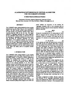
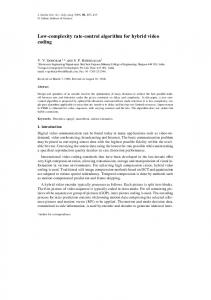
where t r is the amount of the time that has elapsed since t tx (l ) was most recently computed. At events El or E s , rescheduling is done in a way that the earlier of the two times t tx (s) or t tx (l ) is chosen. This rescheduling ensures two objectives: 1) If the current scheduled transmission cannot support current dynamics, the packet transmission is accelerated. 2) If changes in channel load lead to a change in the LIMERIC rate, they are reflected in the next transmission. It is a subtle but important point that the channel load due to accelerated transmissions in some vehicles is offset by LIMERIC adaptation in all vehicles, so that EMBARC ensures to keep the channel load at the desired threshold. In Fig. 1, we show an example of scheduling and rescheduling packet transmissions using our EMBARC algorithm. At event E t , the next packet is scheduled to transmit at 1/ rl time units in the future (i.e., t tx (l ) is denoted by ①). Then an E s event happens and causes a rescheduling of the packet to an earlier time, denoted by position ② (i.e., t tx (s) ), based on high dynamics. Next another E s event further reschedules the packet to an earlier time ③ (i.e., t tx (s) ). At event El the LIMERIC component determines that a later time ④ (i.e., t tx (l ) ) would be acceptable to satisfy the channel load constraint, our EMBARC method transmits the packet at ③.

3.1 Transmissions in EMBARC In EMBARC, three events happen asynchronously. A LIMERIC event ( El ) occurs every  l time units, where a new CBP value is measured and used to compute a rate rl according to Eq. (1). An STE event ( E s ) happens every  s time units, where a candidate transmission time is computed based on the vehicle

Fig. 1.

Sample packet transmissions in EMBARC

In addition, since events E s , El , and E t , are not synchronized with each other, it can happen that right after an event E t , another event E s happens. In a high dynamics scenario or in cases where the channel PER is very high, it is possible that right after a transmission, a node can still have a high STE. A subsequent E s event might suggest that the next transmission should happen right away. But we have imposed a rule in EMBARC, such that no two transmissions may occur within 100 ms. This rule comes from default rate of 10 Hz for BSMs and we want our congestion control algorithm to work in a fashion that transmissions at any time do not go faster than the default rate of 10 Hz.

3.2 STE Component The STE component is responsible for computing the Suspected Tracking Error and determining the next transmission time such that the STE will stay below a specified threshold for the current vehicle dynamics. As in [5], STE is the error with which the HV thinks an RV estimates the HV’s position. When a packet sent by the HV is received correctly by the RV, the RV obtains an accurate estimate of the HV’s position at that particular time. The estimate is in general not exact because the HV GPS sample is both noisy and slightly delayed. In this work, we assume that an RV tracks the HV’s position by extrapolating based on a constant speed and heading model from the most recently received GPS position (i.e. “coasting”). To compute STE, the HV then has to account for different possibilities with regard to which GPS information is the latest that has been delivered to the RV. EMBARC addresses this challenge with an improvement over that presented in [5]. Every packet that is transmitted over a wireless channel has a certain probability of failure (i.e., the channel’s packet error ratio or PER). The HV estimates the PER associated with its transmissions based on the PER it observes for packets sent to it

pk was

employ a binary search algorithm, where search begins from the time when the packet is currently scheduled to transmit. The value of the threshold T’ determines how sensitive EMBARC is to STE. A smaller value leads to transmissions even when the HV exhibits relatively smaller dynamics. GPS noise and a desire to avoid congestion caution against setting the threshold too low. Note that this future-time-based STE is a contribution of this paper; in contrast [5] computes STE only at the current time, and uses a simpler model that coasts from a single prior packet.

3.3 Analysis In EMBARC, in addition to the messages that are transmitted according to the rate determined by the LIMERIC algorithm, there might be extra transmissions that happen because of the vehicle dynamics in the STE component. In this subsection, we model extra transmissions (caused by vehicle dynamics) as a random variable and provide a mathematical analysis on the steady-state rate of the EMBARC algorithm. This analysis shows that the LIMERIC adaptation in each node is impacted by the additional channel load imparted by the aggregate of extra transmissions among all vehicles in the neighborhood. This is a key attribute of EMBARC, reflecting its ability to control the channel load. Thus, each node sends the extra messages dictated by its own dynamics, and collectively all nodes absorb this extra load in equal shares. The original LIMERIC equation is as follows:

r j (t )  (1   )r j (t  1)   (rg  rC (t  1))

(6)

where K

rC (t ) 

 r (t ) j

j 1

(7)

and K is the total number of vehicles in the network. In EMBARC, due to vehicle dynamics, every vehicle may transmit extra packets with rate X j (t ) . We model X j (t ) as a stationary

the

random process with mean  j and variance  2j . In our current

channel PER when k packet was sent, and assuming n packets have been sent so far and the most recent packet is indexed as n, EMBARC computes the HV’s current STE as:

analysis, we assume X j to be independent with respect to time1.

from RVs within a pre-defined range (as in [5]). If th

  (1  pn ) n  pn (1  pn 1 ) n 1  pn pn 1 (1  pn  2 ) n 1 

n

  pi (1  p1 )1 i 2

n 1

n

 (1  pn ) n    pi (1  p j ) j j 1 i  j 1

Further for mathematical tractability, we assume that extra transmissions caused by vehicle dynamics are supplementary to the transmissions that occur due to the LIMERIC rate. This is not entirely accurate, because the occurrence of an early, dynamicsinduced transmission impacts the scheduling of subsequent LIMERIC-induced packets; we comment further on the assumption below. Using this assumption for EMBARC, we can write rC (t ) as:

(5)

where  k , 1  k  n , is the STE computed using constant speed constant heading model assuming the kth packet is the most recent packet that the RV received.

K

rC (t ) 

 (r (t )  X j

j (t ))

Now Eq. (6) can be written as:

_

Note that between two transmissions  is an increasing function of time and we compute the next STE-based transmission time

r j (t )  (1   )r j (t  1)   (rg 

K

 r (t  1))  w(t  1) j

(9)

j 1

_

( t tx (s) ) using binary search to predict the future time when  reaches a specified threshold T’. In particular, HV extrapolates its position in future by constant speed, constant heading coasting from the current position and assumes RV would be coasting it from the last received packet (as in Eq. (5)). It is challenging to obtain t tx (s) by directly solving Eq. (5). Hence, in our work we

(8)

j 1

where w(t )   X j (t ) is a random process representing the aggregate of extra transmissions in the network; it has mean 1

In future we will explore models where random variable X j is

co-related in time.

K

 w    j and variance

 w2 . Note that if extra transmissions

j 1

are independent across vehicles, then 

2 w



Var[rC ] 

K



2 j

.

In the

j 1

interest of exposing the role of the per-node extra rate variances  2j , we use the independence assumption in the remainder of the analysis. Eq. (9) can be written in vector format as: 







r  A r (t  1)   u rg   u w(t  1)

(10)

where 1          A  . .   

 1    . . 

  1   . . 

        .   .  1     

... ... ... ... ... ...



and

u

is a

vector of all ones. For this linear system to be stable, the eigenvalues of A must be within the unit circle. As in [8], if the stability condition   K  2 is satisfied, this linear system will converge in the mean to a unique solution in steady state. Further, in steady-state, each rate converges with mean: E[r j ] 

 (rg   w ) (  K )

(11)

, j  1,2,...K

It can be seen from Eq. (11) that in EMBARC, steady-state rate for each node due to LIMERIC component converges to a lower rate than in [8] to account for the extra transmissions X j . In this manner, EMBARC design ensures to keep the channel load at the threshold. The random nature of aggregate extra transmissions, w(t), also induces random variations in rj(t), even for nodes that have no extra transmissions themselves. The steady state variance in rj can be determined by the following zero-mean system: 





r  A r (t  1)   u w'(t  1)

K 2 2

K



2 j

j 1

(16)

1  (1    K ) 2

Interpretation: Comparing Eqs. 2 and 11, we see that while LIMERIC adapts according to a target load rg, the LIMERIC component of EMBARC adapts according to a new effective target (rg – μw). In other words, it adapts to a fair share of the portion of desired channel load that remains after all extra transmissions. This is precisely what we want. Returning to the original assumption to treat extra transmissions as supplementary to LIMERIC-induced transmissions, Eq. 11 suggests it may be more intuitive to think of it the other way around, i.e. LIMERICinduced transmissions are supplementary to those required by dynamics. Still another interpretation is that each node has a minimum rate required to satisfy STE objectives, and opportunities are allocated in a max-min fair manner that satisfies those constraints. Regardless of interpretation, the analysis above provides an accurate model of steady state mean and variance. We also present MATLAB results to demonstrate the results proved in our analysis. We have set the values of  to be 0.1,  to be 1/150, and rg is set to be 60, equivalent to 1200 msg/sec [8], total number of nodes is set to be 200. Extra transmissions ( X j ) are assumed to be Gaussian distribution with a mean of 0.5 and variance of 1. In Fig. 2, we show the message rate of 4 representative nodes which are initialized to different rates. At steady state all nodes converge to same rate and they have variations in steady state rate. It should be noted that rates plotted in Fig. 2, are same for each node in steady state as they have same distribution of X j . If in practice different vehicles, have different distribution of X j , they would converge to different rates. In Table 1, for various values of mean and variance in X j , we present the comparison results for mean and variance in the steady state rate as predicted by theory (Eqs. 11, 15, 16) and the results that we observe in simulations. It can be seen from Table 1 that results predicted by theory match very closely with simulations.

(12)

where w’(t) = w(t) - μw is a zero-mean process with variance K



2 j

. The covariance matrix can be written as:

j 1



T

C (t )  E[ r (t ) r (t )]

(13)

which can be re-written as, K

C (t )  AC (t  1) AT  (

 j 1

2 j

)  2U

(14)

Xj

where U is a K x K matrix of all ones. This analysis is similar to noise analysis done in [14] and using the discrete-time Lyapunov function we can derive following equations:

2 Var[r j ] 

K



2 j

j 1

1  (1    K ) 2

(15)

Fig. 2. Steady state message rate in EMBARC Mean 0.125 0.25 0.5 1

Simulat ion

Variance

0.25

0.5

1

2

E[r j ]

5.46

5.35

5.12

4.65

Var[rj ]

2.7e-3

5.5e-3

1.1e-2

2.1e-2

Var[rC ]

1.1e+2

2.2e+2

4.3e+2

8.5e+2

Theory

E[rj ]

5.47

5.35

5.12

4.65

Var[rj ]

2.7e-3

5.5e-3

1.1e-2

2.2e-2

Var[rC ]

1.1e+2

2.2e+2

4.4e+2

8.8e+2

Table.1. Mean and variance in steady-state EMBARC rate

4. MOBILITY TRACE Before any simulations can be carried out to evaluate EMBARC, a realistic mobility trace of vehicles is required. As a matter of fact, making transmissions a function of vehicular mobility presents new challenges to the simulation granularity of traffic simulators. Specifically, since vehicular dynamics affect STE, which has an impact on the transmission rate of BSMs, we need a traffic simulator that can model the movement of vehicles in a fine-grained and a realistic way. To the best of our knowledge, none of the existing traffic simulators can validate the realism of the mobility trace in such a microscopic manner. Existing traffic simulators do not use detailed movement of vehicles for calibration and instead they compare the resulted traffic volumes with real data collected from sensors on the road. No guarantees on the detailed movement of vehicles are provided. For our work we used SUMO (which is an open source simulator) to generate mobility traces. We modified SUMO so that the obtained traces are more realistic. In addition, practical GPS devices have a limitation that they cannot detect the precise position of the vehicle. In order to model this limitation, we have introduced GPS noise in the NS-2 simulator (as in [12]).

4.1 Modifications in SUMO and NS-2 The modeling of detailed vehicular movement in a traffic simulator is mainly based on the car-following model and lane change model. The car-following model describes the interaction, i.e., correlation in speed and acceleration, between a vehicle and its leading car in the same lane. The lane-changing model is responsible for determining conditions under which vehicles can change lanes and for executing a lane change. In our work with the SUMO simulator, we found five major challenges that impact the realism of microscopic vehicular movement: 1. Vehicles have perfect knowledge of the environment, including the distance to the neighboring vehicles and their velocities. This leads to very little acceleration for the vehicles while moving on the road. 2. Vehicles have fixed maximum speed, which they desire to achieve, which results in more or less constant speed for a long time. 3. Vehicles move with constant speed within one simulation step (in our simulations we set this step to be 100ms). 4. Lane change is finished in one simulation step, i.e., it is very abrupt. 5. Too few lane changes happen. In real scenarios, drivers cannot have very accurate estimation of headways to leading vehicles unless they are close enough. This is one of the reasons for small changes in the speed of the vehicle while following other vehicles in the same lane. Because of this and because of the fixed maximum speed (challenge 2), SUMO produces mobility traces where vehicles may travel with constant speed. In our work, we modified SUMO by adding noise to the estimation of headways, speeds of leading vehicles, and maximum desired speed. This leads to vibrations in the vehicles’ speed.

As a discrete traffic simulator, SUMO modifies the speed of a vehicle at the beginning of a simulation interval to account for the acceleration during the entire interval. Nevertheless, the speed changes smoothly in real scenarios. We modified SUMO such that the vehicle is able to accelerate continuously throughout the simulation interval. For the lane change model, SUMO moves vehicles to adjacent lanes in one simulation step (as stated in challenge 4). Lane changing is very abrupt in SUMO and it does not even matter how small the simulation step is. As a consequence, it would happen that STE would be very high for that particular simulation step, but after a BSM is transmitted, STE would be again low. This however is not true in realistic movements of the vehicles, where it generally takes 3-5 seconds to change lanes. SUMO implements lateral movement only in discrete steps and we found that it is difficult to improve this feature in SUMO. However, we found that while reading mobility traces from SUMO, the NS-2 implementation ensures that lane changes do not happen abruptly. The reason for challenge 5 is that SUMO executes a lane change only if there is enough gap on the adjacent lane for the vehicle to move onto. However, SUMO calculates the value of this gap required for lane changing to be much larger than required in practice. In reality people may change lanes aggressively even within limited space. We modified SUMO by reducing the scale of the gap needed for executing a lane change, and hence, in our simulations we see more lane changes. By adding these modifications to address the five challenges, we are able to obtain mobility traces where vehicles display realistic dynamics. Further, we also made modifications to the mobility implementation of the NS-2 simulator. We added noise in the mobility traces obtained via SUMO and the distribution of the noise added in speed, heading, and location is the same as in [12]. Additionally, we found out that in NS-2 nodes move with a constant speed and constant heading during each simulation interval. We modified the NS-2 code in a way such that nodes accelerate continuously throughout the simulation interval and they match the corresponding modifications we made in SUMO.

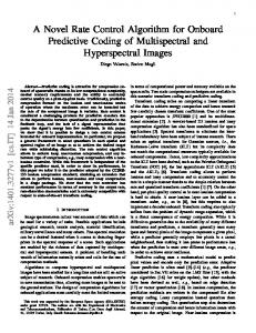
4.2 Road Topology Besides mobility model, the realism of simulations also depends on the accuracy of the wireless channel models. It is well known that fading in wireless environments in urban scenarios (e.g., a crowded intersection) is hard to capture using mathematical formulas. As a consequence, we focus our study on an open highway scenario. As shown in Fig. 3, we configured a highway of 4 km length (3 lanes in each direction), with a section in the middle path set to be winding (radius of the circle in the winding part of the road is set to be 40 meters). The purpose of creating the topology in this manner is to create a scenario where most of the vehicles which are on straight part possess normal dynamics (i.e., fewer variations in the heading of the vehicle), and vehicles on the winding part have higher dynamics (i.e., heading of the vehicle is varying quite fast). We expect the STE to be much higher on the winding part. The length of the winding part is around 375m. The 3 lanes on the highway have an average desired speed for the vehicles set to be 19m/s, 18m/s, and 17m/s from the fastest lane (leftmost lane) to the slowest lane (rightmost lane).

Fig. 3.

Road topology for simulations

compoenent)

5. NUMERICAL RESULTS In this section, we evaluate the performance of EMBARC using the NS-2.34 simulator. We compare the performance of EMBARC with fixed 10Hz transmission, LIMERIC (with PULSAR), IVTRC and IVTR-PC (as in [6]). Our primary metric for performance comparison is 95% TE (i.e. 95th percentile of all TE samples in the simulation), where TE is the error between the HV’s true position and the RV’s perception of the HV position. We assume that the RV extrapolates the HV position from the last received BSM using a constant-speed constant-heading coasting model. TE is computed every 100 msec. We also provide results for average message rate for the various algorithms. Also, since TE depends both on the HV’s dynamics and on the frequency of successfully delivering BSMs to receiving nodes, it is helpful to also analyze Packet Error Ratio (PER) and mean Inter-Packet reception Gap (IPG) results. PER is an indicator of channel quality and for a given number of nodes mean IPG is inversely proportional to throughput. We ran our simulations for four density scenarios (S1 – S4) with 100, 500, 1000 and 1500 nodes, respectively, on the 4 km road shown in Fig. 3. Although the average desired speeds of nodes in these scenarios follow the same distribution in each scenario (i.e., 19m/s 18m/s 17m/s from the fastest lane to the slowest lane.), the actual speeds differ across scenarios. This happens because in SUMO traffic speed decreases as traffic density increases. We consider wireless channel fading to be Nakagami distributed. NS2 supports the implementation of Nakagami fading and we chose the fading parameters as in [7]. The default transmit power is set to 10dBm which corresponds to a 500m transmission range in NS2. The comprehensive list of simulation parameters is as follows: Common Parameter

Value

IVTRC

Value

Noise floor

-99dBm

T

0.3m

Carrier sense threshold

-96dBm

α

50

Packet reception SINR (for 6 Mbps packet)

7dBm

Tguard

300msec

Payload size

350bytes

σ

100msec

Transmission rate

6Mbps

IVTR-PC

Transmission power

10dBm2

Lmin

100m

GPS update frequency

10Hz

Lmax

500m

Maximum allowed BSM rate

10Hz

Umin

0.4

Minimum allowed BSM rate

1Hz

Umax

0.8

LIMERIC

EMBARC

δ

200ms

T’

0.2m

rg

60%

rg (LIMERIC component)

60%

β

0.0025

β (LIMERIC

0.0025

2

We chose power to be 10 dBm as it is equivalent to 500 meters transmission range in NS-2 which is an adequate range for DSRC.

α

0.1

α (LIMERIC compoenent)

0.1

l

200msec

s

100msec

Table.2. NS-2.34 Simulation Parameters

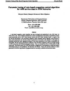
5.1 Rate Adaptation In this subsection, we analyze the transmission interval behavior of three rate-control protocols: IVTRC, LIMERIC and EMBARC, by investigating inter-transmission time (ITT, i.e., time between two consecutive packet transmissions). We select an example node from Scenario S2 and plot its, speed and heading as it moves from the straight to the winding part of the road and back again. It can be observed that between 7 and 27 seconds the node’s heading changes rapidly, indicating that it is on the winding part of the road in that interval.

Fig. 4.

Heading and speed of the example node

In Fig. 5, we plot the histogram of ITT for these protocols. The left column contains the distribution of ITT when the vehicle travels on the winding part of the road and the right column has the distribution for the straight part of the road. It should be noted that in order to avoid edge effects, in this paper the straight road results are not from the entire straight part of the road. Straight part results are only from the straight part section located in ± 500 meters from the center of the road. Since vehicle travels on the straight part of the road, with mostly constant heading and constant speed, in Fig. 5b we see that most of IVTRC’s transmissions on the straight road are separated by the guard interval (Tguard = 300 msec). A few smaller intervals occur due to occasional lane changes and noise in the GPS measurements. From Fig. 5a, we can see that IVRTC transmits with a 200 msec interval approximately 30% of the time on the winding part of the road, due primarily to heading changes, but the incidence of 100 msec intervals is not much greater than on the straight road. In Figs. 5c and 5d, we see ITT results for LIMERIC, in which transmission rate depends only on channel load. Hence, ITT for both straight and winding parts of the road are similar. In Scenario S2, LIMERIC converges to 4.8 Hz (Table 3) and as expected we see ITT tightly bunched around 208 msec in Figs. 5c and 5d. Our EMBARC algorithm takes both dynamics and channel load into account. As a consequence, when the example vehicle moves on the winding section (Fig. 5e) where the STE grows more rapidly, the distribution of ITT shifts to smaller values (compared with Fig. 5c), with 18% of samples at the minimum 100 msec. In order to make up for the extra transmissions, the LIMERIC component of EMBARC converges to a slightly lower rate than in the pure LIMERIC algorithm, so the largest ITT in Fig. 5e is higher. We see in Fig. 5f, when the vehicle travels on the straight part, the spread of ITT is larger with EMBARC than with

LIMERIC in Fig. 5d. Most of the samples are tightly bunched, indicating they are scheduled by the LIMERIC component.

5.2 Performance Results In this subsection, we provide performance results of our EMBARC algorithm, compared with fixed 10 Hz, LIMERIC, IVTRC and IVTR-PC. We first provide results for our primary metric: 95% TE. As TE is higher when vehicles are moving on winding part of the road, we mostly focus there. We also provide results for PER and mean IPG for various algorithms. Scenario S1 (100 nodes): First, in Figs. 6-9, we plot 95% TE results against TX-RX distance for our four node density scenarios S1-S4 (respectively 100, 500, 1000, 1500 vehicles on the 4 km road), for transmitters on the winding road. From Fig. 6, we can see that for scenario S1, EMBARC, LIMERIC, and 10 Hz perform the same, and they have much lower TE than IVTRC and IVTR-PC at distances above 150 m [Note: bin 25 covers 0-50 meters, etc.]. For this case EMBARC and LIMERIC converge to 10 Hz. IVTRC and IVTR-PC converge to a much lower rate and are underutilizing the channel. Higher rates mean higher PER and hence, we observe in Fig. 11, that PER is slightly higher for EMBARC, LIMERIC and 10 Hz as compared to IVTRC and IVTR-PC. Average IPG (in Fig. 15) is much lower for EMBARC, LIMERIC and 10 Hz, i.e., they have better throughput.

Fig. 5. Histogram of ITT for S2 (500 nodes) using different rate-control protocols. Subfigures (a) – (b) show results for IVTRC, (c) - (d) for LIMERIC, and (e) - (f) are for EMBARC. Table 3 presents the average message rate across all nodes for the three rate-control protocols. The average LIMERIC rate depends only on node density (scenario) and not on road segment type. For IVRTC, rate is approximately independent of node density, and is slightly higher on the winding part compared to the straight part. EMBARC takes both channel load and road topology into account. It converges to higher rates with lower node densities and always has higher average rates on the winding part than the straight part. We also notice that in scenarios S2, S3, and S4 EMBARC’s rate on straight part is less than LIMERIC rate. Vehicles while being on the winding part have dynamics which causes extra transmissions due to STE component in EMBARC. This can increase channel load and hence, LIMERIC component reduces the message rate so that channel load can be maintained at the threshold. The design of EMBARC ensures that the increased transmission due to dynamics experienced by certain vehicles is compensated by the reduced rate of the LIMERIC component for all the vehicles. As a result, we see that the average rate on straight part in EMBARC is lower than the rate of LIMERIC algorithm. Vehicles on the straight part of the road “pay the price” for extra transmission on winding part and channel load is maintained at the target threshold. Scenarios S1 S2 S3 S4

Road sections

IVTRC

LIMERIC

EMBARC

Winding

3.7Hz

10.0Hz

10.0Hz

Straight

3.5Hz

10.0Hz

10.0Hz

Winding

3.8Hz

4.8Hz

5.1Hz

Straight

3.5Hz

4.8Hz

4.8Hz

Winding

3.8Hz

2.7Hz

4.0Hz

Straight

3.6Hz

2.7Hz

2.5Hz

Winding

3.7Hz

1.9Hz

2.7Hz

Straight

3.6Hz

1.9Hz

1.8Hz

Table.3. Average transmit rate used by nodes while on the winding and straight section of the road.

Scenario S2 (500 nodes): We observe in Fig. 7 that 10 Hz performs a bit better than EMBARC up to 200 m, and then EMBARC is best as the performance of 10 Hz deteriorates. EMBARC’s average rate for the winding part (5.1 Hz from Table 3) is just over half of the fixed 10 Hz algorithm. EMBARC transmits its messages intelligently, i.e. extra transmissions are allocated when STE is high, and it also has a much lower PER than 10 Hz, as seen in Fig. 12. The higher PER slope for 10 Hz in Fig. 12 reflects a higher hidden-node loss probability due to the fact that the hidden nodes also transmit at 10 Hz. The STE-based transmission and lower PER for EMBARC more than make up for its lower rate. EMBARC also outperforms LIMERIC, IVTRC and IVTR-PC. LIMERIC converges to a higher rate (4.8 Hz) than IVTRC and has better performance than IVTRC and IVTR-PC. Another interesting observation from Fig. 7 is that for this node density channel load is high enough (CBP > Umin = 0.4) to trigger power control, and hence IVTRC and IVTR-PC perform differently. We observe that IVTRC performs better than IVTRPC. Reducing the power in IVTR-PC has a harmful effect on 95% TE performance, especially at higher distance. At lower distances power control reduces the congestion and one might expect it to have better PER, TE performance. But as we observe in Fig. 7 and Fig. 12, power control does not even help at lower distances. This is because of the capture effect in 802.11 (which NS-2 models), which permits reception of some near transmissions even they overlap another packet. As a result, we found that IVTR-PC performs worse than IVTRC for all the distances.

Fig. 6.

95% TE for nodes in S1 on winding part of the road

LIMERIC has lower 95% TE than IVTRC. This is because from Fig. 14, we see that LIMERIC takes channel load into account and for this very dense scenario has the lowest PER. IVTRC cannot transmit less frequently than Tguard = 300 msec, resulting in higher PER. EMBARC transmits more than LIMERIC on both road segments. Compared to IVTRC EMBARC is higher on the winding part and lower on the straight part. But, EMBARC’s 95% TE is better than both LIMERIC and IVTRC at all distance bins. On the critical winding part this is due to more intelligent transmission scheduling. Fig. 7.

95% TE for nodes in S2 on winding part of the road

Fig. 8.

95% TE for nodes in S3 on winding part of the road

In Fig. 10, we also show 95% TE result for straight part of the road for scenario S2. Here, we can observe that even on the straight segment EMBARC is a bit worse than 10Hz upto 200 meters, but outperforms all the other algorithms.

Fig. 11. PER for nodes in S1 on winding part of the road

Fig. 9.

95% TE for nodes in S4 on winding part of the road Fig. 12. PER for nodes in S2 on winding part of the road

Fig. 10. 95% TE for nodes in S2 on straight part of the road Scenarios S3 and S4 (1000 and 1500 nodes): We observe in Fig. 8 that EMBARC significantly outperforms all the other algorithms for S3. After EMBARC, IVTRC performs better than LIMERIC, which performs better than 10 Hz. From Table 3, we can see EMBARC has the highest rate among the three variable-rate protocols (4.0 Hz) on the winding road, and LIMERIC has the lowest (2.7 Hz). But, all are below 10 Hz, so TE performance is not monotonic with rate. We can also see from Fig. 17 that EMBARC has lowest average IPG, and thus highest throughput, for most distances. We see similar trends in 95% TE results in Fig. 9 for Scenario S4. However, we see that above 250 meters

Fig. 13. PER for nodes in S3 on winding part of the road

Fig. 14. PER for nodes in S4 on winding part of the road

6. CONCLUSIONS

Fig. 15. IPG for nodes in S1 on winding part of the road

Improving the performance of DSRC in dense networks is critical to its success in the future Intelligent Transportation System. Congestion control is therefore a key technology. The primary philosophy is to control message transmissions to keep the channel load operating at a non-congested level. In this paper, we propose a novel approach for congestion control called EMBARC. It adjusts the BSM transmission rate based on both channel load and vehicular dynamics. On one hand, EMBARC inherits the advantage from LIMERIC of high throughput independent of number of neighbors. On the other hand, it is able to schedule extra packet transmissions using an intelligent futurelooking TE estimate. In this way, vehicles that are more difficult to track will transmit more BSMs, so that others track them with high accuracy even in dense traffic scenarios. EMBARC represents an important bridge between two previously separated approaches to congestion control.

7. REFERENCES

Fig. 16. IPG for nodes in S2 on winding part of the road

Fig. 17. IPG for nodes in S3 on winding part of the road

Fig. 18. IPG for nodes in S4 on winding part of the road

5.3 Summary From the above simulation results, we have demonstrated the performance advantage of EMBARC. At lower densities (scenario S1), EMBARC can transmit at higher rates like LIMERIC and avoids the problem of underusing the channel as in IVTRC. At medium and high densities, EMBARC is able to adapt its rate because of the LIMERIC component and hence does not have very high PER. And at the same time it transmits more when STE is higher (as IVTRC) and hence, would reduce the TE for a highly dynamic vehicle as compared to the LIMERIC protocol. It can be observed from results that across all node densities EMBARC outperforms all the other algorithms.

[1] J. B. Kenney, “Dedicated Short Range Communications (DSRC) Standards in the United States”, Proc. of the IEEE, 2011. [2] H. Lu, C. Poellabauer, "Balancing Broadcast Reliability and Transmission Range in VANETs," IEEE VNC, Dec. 2010 [3] Bilstrup, K.; Uhlemann, E.; Strom, E.G.; Bilstrup, U.; , "Evaluation of the IEEE 802.11p MAC Method for Vehicleto-Vehicle Communication," IEEE VTC-Fall, Sept. 2008. [4] Torrent-Moreno, M.; Mittag, J.; Santi, P.; Hartenstein, H.; , "Vehicle-to-Vehicle Communication: Fair Transmit Power Control for Safety-Critical Information," IEEE Trans. on Veh. Tech., vol.58, no.7, pp.3684-3703, Sept. 2009 [5] Ching-Ling Huang; Fallah, Y.P.; Sengupta, R.; Krishnan, H.; "Intervehicle Transmission Rate Control for Cooperative Active Safety System," Intelligent Transportation Systems, IEEE Transactions on , vol.12, no.3, pp.645-658, Sept. 2011 [6] C.-L. Huang, et al., “Adaptive Intervehicle Communication Control for Cooperative Safety Systems”, IEEE Network, vol. 24, no. 1, pp. 6-13, Jan.-Feb. 2010. [7] S. Sharafkandi, G. Bansal, J. Kenney, and D. Du, “A Novel use of EDCA to Improve Vehicle Safety Communication,” IEEE VNC, Nov. 2012. [8] J. Kenney, G. Bansal, and C. Rohrs, “LIMERIC: A Linear Message Rate Control Algorithm for Vehicular DSRC Systems,” 8th ACM VANET Workshop, Sept. 2011. [9] Lin Yang; Jinhua Guo; Ying Wu; , "Channel Adaptive One Hop Broadcasting for VANETs," IEEE ITSC, Oct. 2008. [10] Tielert, T.; Jiang, D.; Qi Chen; Delgrossi, L.; Hartenstein, H.; "Design methodology and evaluation of rate adaptation based congestion control for Vehicle Safety Communications," IEEE VNC, pp.116-123, Nov. 2011. [11] Ching-Ling Huang; Fallah, Y.P.; Sengupta, R.; Krishnan, H.; "Information Dissemination Control for Cooperative Active Safety Applications in Vehicular Ad-Hoc Networks," IEEE GLOBECOM, pp.1-6, Nov. 30 - Dec. 4, 2009. [12] S. Rezaei, R. Sengupta, H. Krishnan, X. Guan “Adaptive Communication Scheme for Cooperative Active Safety System,” WoCo, 2008. [13] R. K. Schmidt, T. Leinmüller, and G. Schäfer, “Adapting the Wireless Carrier Sensing for VANETs,” in WIT, Hamburg, Germany, March 2010. [14] G. Bansal, J. Kenney, and C. Rohrs, “LIMERIC: A Linear Adaptive Message Rate Algorithm for DSRC Congestion Control” under review in IEEE Tran. On Veh. Tech., 2013.