{jhma, pcyuen}@comp.hkbu.edu.hk ... cannot be solved analytically, so the solution may not be ...... [16] K. Nandakumar, Y. Chen, S. C. Dass, and A. K. Jain.
Linear Dependency Modeling for Feature Fusion Andy J H Ma and Pong C Yuen Department of Computer Science, Hong Kong Baptist University Kowloon Tong, Hong Kong {jhma, pcyuen}@comp.hkbu.edu.hk
Abstract This paper addresses the independent assumption issue in fusion process. In the last decade, dependency modeling techniques were developed under a specific distribution of classifiers. This paper proposes a new framework to model the dependency between features without any assumption on feature/classifier distribution. In this paper, we prove that feature dependency can be modeled by a linear combination of the posterior probabilities under some mild assumptions. Based on the linear combination property, two methods, namely Linear Classifier Dependency Modeling (LCDM) and Linear Feature Dependency Modeling (LFDM), are derived and developed for dependency modeling in classifier level and feature level, respectively. The optimal models for LCDM and LFDM are learned by maximizing the margin between the genuine and imposter posterior probabilities. Both synthetic data and real datasets are used for experiments. Experimental results show that LFDM outperforms all existing combination methods.
1. Introduction Many computer vision and pattern recognition applications face the challenges of complex scenes with clustered backgrounds, small inter-class variations and large intraclass variations. To solve this problem, many algorithms have been developed to extract local or global discriminative features e.g. SIFT [14], HOG [5], Laplacianfaces [10]. Instead of extracting a high discriminative feature, fusion has been proposed and the results are encouraging. One popular approach to make use of all features is to train a classifier for each of them, and then combine the classification scores to draw a conclusion. While many classifier combination techniques [11, 12, 16] have been studied and developed in the last decade, it is a general assumption that classification scores are conditionally independent distributed [12, 16]. With this assumption, the joint probability of all the scores can be expressed as the product of the marginal probability. the conditionally independent as-
sumption could simplify the problem, but may not be valid in many practically applications. In [17, 20], instead of taking the advantage of conditionally independent assumption, the classifier fusion methods are proposed by estimating the joint probability distribution of multiple classifiers and performance is improved. However, when the number of classifiers is very large, it needs numerous data to accurately estimate the joint distribution estimation [24]. On the other hand, Terrades et al. [25] proposed to combine classifiers in a non-Bayesian framework by linear combination. Under dependent normal assumption (DN), they formulated the classifier combination problem into a constraint quadratic optimization problem. Nevertheless, the objective function in DN method cannot be solved analytically, so the solution may not be optimal. Moreover, when the number of classifiers is large, DN method is very computationally expensive. Apart from these methods, classifier ensemble methods [22] can implicitly model dependency as well. Most of the classifier ensemble methods aim at determining the correct weighting for linear classifier combination to improve the classification performance, e.g. LPBoost [6] and its muticlass generation [8]. All the above-mentioned methods perform the fusion based on classifier scores and implicitly assume that the feature dependency can be reflected by the classifier dependency. So feature level dependence modeling should be performed directly. The key problem is that the dimension of feature is normally large and it is very hard to estimate the joint probability distribution. Multiple Kernel Learning (MKL) [2] can be considered as a feature level fusion method and finds the optimal combination of features. To solve the complexity problem, a fast method [21] is proposed. However, the MKL methods do not consider the feature dependency explicitly as well. In this paper, we develop a novel framework for dependency modeling, and propose two methods, namely Linear Classifier Dependency Modeling (LCDM) and Linear Feature Dependency Modeling (LFDM), at classifier level and feature level respectively. Inspired by the Bayesian model
with independent assumption, we prove that linear combination of the posterior probabilities of each classifier can model the dependency under mild assumptions, which is LCDM. It is believed that dependency in feature level is more effective than that in classifier, so we generalize LCDM to feature level and propose LFDM. Finally, the optimal models for LCDM and LFDM are obtained by solving a standard linear programming problem, which maximizes the margins between the genuine and imposter posterior probability. The contributions of this paper is two-fold. • We prove that feature dependency can be modeled by a linear combination of the posterior probabilities of each feature/classifier under mild assumptions. This conclusion is obtained by adding small dependency terms to the naive Bayesian probability, expanding the product probability and neglecting the terms of order two and higher. • We propose two novel LCDM and LFDM algorithms for modeling the dependency in classifier level and feature level, respectively. LCDM is developed based on linear classifier combination property, and LFDM is derived by generalizing LCDM to feature level. The optimization problems of LCDM and LFDM are formulated as a standard linear programming problem, which therefore, has an analytical solution. Moreover, LCDM and LFDM are derived without any assumption on classifier and feature distribution. This paper is organized as follows. We will first give a review on the classifier combination model under independent assumption in Section 2. Section 3 will report our proposed method. Experimental results and conclusion are given in Sections 4 and 5 respectively.
2. Review of Classifier Combination Model under Independent Assumption In [12], a theoretical framework was developed for combining classifiers. According to Bayesian theory, under the assumption that classifier scores are distributed independently, the posteriori probability is given by [12] QM Pr(ωl ) m=1 Pr(~xm |ωl ) Pr(ωl |~x1 , · · · , ~xM ) = Pr(~x1 , · · · , ~xM ) (1) M Y P0 Pr(ωl |~xm ) = Pr(ωl )M −1 m=1 QM
Pr(~ x )
m m=1 where P0 = Pr(~ x1 ,··· ,~ xM ) . Product rule was then derived by (1). Moreover, taking additional assumption that posteriori probability of each classifier will not deviate dramatically from the prior probability, i.e.
l Pr(ωl |~xm ) = Pr(ωl )(1 + δm )
(2)
l where δm is a small term, Sum rule was induced [12]. Based on Product rule and Sum rule, Kittler et al. [12] justified
that the commonly used classifier combination rules, i.e. Max, Min, Median and Majority Vote, can be derived. It was shown that Sum rule outperforms other classifier combination schemes in their experiments.
3. Linear Dependency Modeling With conditionally independent assumption, the posteriori probability can be computed as in (1). However, as the discussed in Section 1, this assumption may not be true in many practical applications. Thus, in this paper, we remove this independent assumption and study dependent cases. In this section, we propose a new linear dependency modeling method to model the dependency. We first derive the model in classifier level and then proceed to feature level. Finally, we present a learning method to learn the optimal model.
3.1. Linear Dependency Modeling in Classifier Level Let us consider the case that there exists m′ , s.t. Pr(ωl |~xm′ ) = 0 and Pr(ωl |~xm ) = 1 for 1 ≤ m ≤ M , m 6= m′ . In this case, there are M − 1 classifiers giving strong confidences on assigning the class label as ωl , and one classifier concludes other label. When M ≫ 1, we can ignore the m′ classifier giving Pr(ωl |~xm′ ) = 0, and the posterior probability Pr(ωl |~x1 , · · · , ~xM ) is expected to be large. However, with conditionally independent assumption, from (1), the posterior probability by all classifiers becomes zeros. This means, in this case, the posterior probability only depends on one single classifier which satisfies Pr(ωl |~xm′ ) = 0 and the other classifiers will not have any contribution on it. In order to avoid the posterior probability to be zero and dominated only by one classifier, we add a term to Pr(ωl |~xm′ ). This action also affect the posterior probability of some classifiers. So, for all classifiers, we add a term to model the dependency between them. Moreover, the classifier scores with dependency terms cannot deviate much from the original scores. Otherwise the original decision by each single classifier will take little effect on the final decision. Therefore, the values of the dependency terms must l be small. In addition, it is believed that δm , m = 1, · · · , M from (2) should be small values [12]. Suppose small del l l pendency terms are defined by αm Pr(ωl )δm , where αm are the weights to model the dependency between classifierl s. αm = 0 means that classifier m is independent with l the other classifiers. And αm 6= 0 suggests that classifier m is dependent with the other classifiers except those with l l αm ′ = 0. Moreover, we restrict that |αm | ≤ 1, so that l l l l l |αm Pr(ωl )δm | ≤ |Pr(ωl )δm |. By adding αm Pr(ωl )δm to
Pr(ωl |~xm ) in (1), the posterior probability becomes
it can be rewritten as
Pr(ωl |~x1 , · · · , ~xM ) =
P0 Pr(ωl )M −1
M Y
l l (Pr(ωl |~xm ) + αm Pr(ωl )δm )
(3)
m=1
With (2) and (3), we get Pr(ωl |~x1 , · · · , ~xM ) = P0 ∗ Pr(ωl )
M Y
l l (1 + βm δm ) (4)
m=1 l where βm
l αm +1, 0
= ≤ ≤ 2. If we expand the product term in the right hand side of (4) and neglect the terms of second and higher orders, the posterior probability becomes M X
l l βm δm ) (5)
m=1 l Substituting δm by (2) into (5), we obtain
Pr(ωl |~x1 , · · · , ~xM ) = P0 ∗ (
M X
(7)
With this representation (7), each element in feature vector can be viewed as a single classifier. Similar to the analysis in Section 3.1, the dependency term for each xmn can be l l l l written as αmn Pr(ωl )δmn , where αmn satisfies |αmn | ≤ 1, and the posterior probability analogous to (3) is given by Pr(ωl |x11 , · · · , x1N1 , · · · , xM 1 , · · · , xM NM )
l βm
Pr(ωl |~x1 , · · · , ~xM ) = P0 ∗ Pr(ωl )(1 +
Pr(ωl |~x1 , · · · , ~xM ) = Pr(ωl |x11 , · · · , x1N1 , · · · , xM 1 , · · · , xM NM )
l βm Pr(ωl |~xm ) + Pr(ωl )(1 −
M X
M N m Y Y P0′ l l (Pr(ωl |xmn ) + αmn Pr(ωl )δmn ) Pr(ωl )M −1 m=1 n=1
(8) QM
QNm
Pr(x
)
mn n=1 m=1 where P0′ = . Following the same Pr(~ x1 ,··· ,~ xM ) derivation procedures from (3) to (6) in Section 3.1, the posterior probability with dependency modeling in feature level can be written as
Pr(ωl |x11 , · · · , x1N1 , · · · , xM 1 , · · · , xM NM ) l βm ))
(6)
m=1
m=1
=
PM
l At last, the summation of weights m=1 βm should be PM l to normalized respect to class label l, so we set m=1 βm be a constant related to l. When the independent assumption PM l l = M. holds, βm = 1 for all m, which results in m=1 βm In turn, the Linear Classifier Dependency Model (LCDl M) is derived in (6) with the constraints 0 ≤ βm ≤ 2, PM l β = M . m=1 m
3.2. Linear Dependency Modeling in Feature Level Given the feature vectors ~x1 , · · · , ~xM , where ~xm = (xm1 , · · · , xmNm ), Pr(ωl |~xm ) can be computed by the joint probability Pr(xm1 , · · · , xmNm |ωl ). Since ~xm are normally high dimensional vectors, it needs numerous samples to estimate the joint probability accurately [24]. In general, the probability is hard to determine accurately. In classifier combination methods [12, 25], the posterior probabilities Pr(ωl |~xm ) are viewed as scores calculated from certain classifiers, such as support vector machines (SVM). The scores can be positive or negative. However, probability distributions, Pr(ωl |~xm ) cannot be negative, so classification scores may not be the best way to infer the probabilities Pr(ωl |~xm ). On the other hand, classifiers are trained individually for a single feature and optimal classifiers can be obtained under certain criteria. There is no guarantee that they are optimal after fusion. Let us consider the posterior probability by all classifiers Pr(ωl |~x1 , · · · , ~xM ). Given the feature vectors ~x1 , · · · , ~xM ,
= P0′ ∗ (
Nm M X X
l γmn Pr(ωl |xmn ) + Pr(ωl )(1 − K))
(9)
m=1 n=1
PM l l where K = m=1 Nm , and γmn = αmn + 1 satisfies l 0 ≤ γmn ≤ 2. This gives the Linear Feature Dependency Model (LFDM). Comparing with LCDM, the advantages of LFDM are three-fold. First, (6) relies on classifier computation. It needs efforts to choose the best classifiers. Second, dependency modeling in feature level provides more information than that in classifier level. This is because classification scores are inferred from features while the inverse may not be feasible. Third, since Pr(ωl |xmn ) is one dimensional distribution, much less samples are required to estimate the density accurately [24].
3.3. Learning Optimal Linear Dependency Model The optimal LCDM and LFDM can be learned by different criteria to optimize the classification performance. In this section, we consider the marginal criterion, and give detailed derivations on how to learn the optimal LFDM. Similar derivations can be applied to LCDM. Let the training samples and the corresponding labels be denoted by ~xj = (xj11 , · · · , xj1N1 , · · · , xjM 1 , · · · , xjM NM ) and yj , j = 1, · · · , J, respectively. If all the training samples are correctly classified, Pr(yj |xj ) > maxωl 6=yj Pr(ωl |xj ). Under this condition, the difference between the genuine and imposter probabilities Pr(yj |xj ) − maxωl 6=yj Pr(ωl |xj ) is large. In turn, the performance will be good. Considering the marginal criterion, and inspired
by LPBoost [6] and its multiclass generalization [8], the objective function to learn the best model is defined as J 1 X X l ξj νJ j=1
min − a +
γ,a,ξ
ωl 6=yj
j
s.t. i) Pr(yj |x ) − Pr(ωl |xj ) ≥ a − ξjl , ∀j, ωl 6= yj
(10)
ii) Pr(ωl |xj ) ≥ 0, ∀j, ωl , iii) ξjl ≥ 0, ∀j, ωl
The optimal LFDM is learned by (12). Similarly, the optimal LCDM can be obtained by applying (6) into (10), and follow the same derivation procedures from (10) to (12). The optimization problems for LCDM and LFDM are standard linear programming problems. Thus, the solution can be determined by any off the shelf techniques, e.g. [15]. Since our experiments are performed in the Matlab environment, a Matlab build-in function is employed.
3.4. Remarks where ν is a constant parameter, ν ∈ (0, 1). Let us denote Pr(ωl |xjmn ) in (9) as pj,l mn . Substituting (9) into (10) and ignoring P0′ as a constant respective to class label, the optimization problem (10) becomes min − a +
γ,a,ξ
s.t. i)
J 1 X X l ξj νJ j=1 ωl 6=yj
Nm M X X
yj j,yj γmn pmn
m=1 n=1
−
Nm M X X
(11) l l γmn pj,l mn ≥ a − ξj , ∀j, ωl 6= yj
m=1 n=1
ii)
Nm M X X
l γmn pj,l mn ≥
m=1 n=1
K −1 , ∀j, ωl , iii) ξjl ≥ 0 L
where L is the number of classes. Optimization problem (11) is theoretically sound and purely derived from (10) mathematically. However, in practice, there may not be any feasible solution to (11). If there 1 0 ,l0 exists j0 and l0 such that pjmn < L1 − KL , ∀m, n, then PM PNm l j0 ,l0 K−1 it has m=1 n=1 γmn pmn < L . This means, the inequality in constraint ii) cannot be satisfied for j0 and l0 , so there is no feasible solution to the optimization problem (11). Thus, to make sure that feasible solutions exist, we drop the constraint ii) in (11). l Adding the normalization and range constraints to γmn as mentioned in Section 3.2, the final optimization problem becomes min − a +
γ,a,ξ
s.t. i)
J 1 X X l ξj νJ j=1 ωl 6=yj
Nm M X X
yj j,yj γmn pmn
Nm M X X
l l γmn pj,l mn ≥ a − ξj , ∀j, ωl 6= yj
m=1 n=1
ii) ξjl ≥ 0, ∀j, ωl , iii)
4. Experimental Results In this section, we evaluate the two proposed methods, namely Linear Classifier Dependency Modeling (LCDM) and Linear Feature Dependency Modeling (LFDM), with synthetic data as well as three real image/video databases. The real image/video databases are Oxford Flowers [18], Weizmann [9], and KTH [23]. First, we briefly introduce the databases and the experiment settings. Then, we compare the proposed LCDM with state-of-art classifier combination methods with synthetic data and the Flowers database in Sections 4.2 and 4.3 respectively. Finally, we compare LFDM with feature-level combination methods on Weizmann and KTH action databases in Section 4.4.
4.1. Database and Experiment Setting
m=1 n=1
−
1. LFDM gives the optimal feature combination by modeling dependency between features, so LFDM is an optimal feature-level combination method. 2. LCDM gives the optimal classifier combination by modeling dependency between classifiers, so LCDM is an optimal classifier-level fusion method. 3. Considering the probabilities pj,l mn in (12) as classification scores, the derived formulation (12) looks like the objective function of LP-B in [8]. Though the goal and the starting points of this paper are different from boosting methods, we come up with a similar optimization probl lem with different constraints (0 ≤ γmn ≤ 2). Boosting methods aim at finding the optimal combination of classifiers, while our objective is to model the feature depenl dency. Without the constraint 0 ≤ γmn ≤ 2, when the number of classifiers is large (for LCDM) or the fusion is l performed in feature level (for LFDM), γmn can increase to a large value. This makes the derivation from (4) to (5) l be invalid. Thus, the constraint 0 ≤ γmn ≤ 2 is very important for dependency modeling.
Nm M X X m=1 n=1
l iv) 0 ≤ γmn ≤ 2, ∀l, m, n
l γmn = K, ∀l
(12)
Synthetic data: Similar to [1, 25], four types of classifier distributions, namely Independent Normal (IndNormal), Dependent Normal (DepNormal), Independent NonNormal (IndNonNor), Dependent Normal (DepNonNor) are used to evaluate LCDM and other classifier combination methods. For each distribution, 2000 samples (500 positive and 500 negative for training and testing) of 40 dimension-
s which simulate 40 classifiers are randomly generated by Matlab built-in function. In order to avoid the possibility that the results could be influenced by the random number generation, we run the experiments 200 times. For multiclass methods, LP-B and the proposed LCDM method, we estimate the genuine and imposter posterior probabilities by each classifier, i.e. Pr(+|sm ) and Pr(−|sm ), where sm represent the scores, as in [3]. Oxford Flower Database: This database contains 17 different types of flowers with 80 images per category [18]. Some example images are shown in Fig. 1 (a). Seven different types of features including shape, color, texture, HSV, HoG, SIFT internal, and SIFT boundary, are extracted using the method reported in [18, 19]. Distance matrices of these features and three predefined splits of the database (17 × 40 for training, 17 × 20 for validation, and 17 × 20 for testing) are available on their website1 . We follow the experiment settings in [8]. 5-fold cross validation (CV) in the training set is used to select the best classifier for each feature. The CV outputs are used to train the weights for classifier combination. The best parameter ν is selected from {0.05, 0.1, . . . , 0.95} on the validation set with the Kernel matrices exp (−λ−1 d(x, x′ )), where d is the distance and λ is the mean of pairwise distances. Weizmann database: Weizmann database contains 93 videos from 9 persons, each performing 10 actions [9]. Example images from the videos are shown in Fig. 1 (b). Since the size of the database is small, we use nine-fold CV to evaluate the proposed method. In each validation, data from 8 persons are used to train classifiers and the best combinations, as well as estimate the posterior probability Pr(ωl |xmn ) in LFDM by [3]. The average recognition rate is recorded. KTH database: There are 25 subjects performing 6 actions under 4 scenarios [23] in KTH database. Example images from the videos are shown in Fig. 1 (c). We follow the common setting [23] to separate the video set into training (8 persons), validation (8 persons), and testing (9 persons) sets. Each classifier and combining classifiers are trained using the training set, and selected by the validation. The range of ν is 0.1 to 0.9 with 0.1 incremental step. And the posterior probability in LFDM is estimated on training and validation sets by [3]. Classifiers: For classifier combination methods, we use the Support Vector Machine (SVM) Toolbox provided by [4] to train classifiers for each feature. The parameter introduced in the soft margin SVM is selected from the range C ∈ {0.01, 0.1, 1, 10, 100, 1000} for all the combination methods. 1 http://www.robots.ox.ac.uk/
vgg/data/flowers/17/index.html
Figure 1. (a) Example images from Flower database [18]. Images from the same columns are from the same classes, (b) Example images from videos representing all the 10 actions in Weizmann [9], (c) Example images from videos in KTH [23]. All 6 actions and 4 scenarios are presented.
Feature Extraction: For Weizmann and KTH databases, we adopt the bag-of-features approach and extract 8 types of features for the videos. First, space-time interest points are detected by [7] from each video. For each interest point, 8 local descriptors, namely 1) intensity, 2) intensity difference, 3) histograms of optical flow (HoF) without grid, 4) histograms of gradient (HoG) without grid, 5) HoF with 2D grid, 6) HoG with 2D grid, 7) HoF with 3D grid and 8) HoG with 3D grid, are generated based on 9 × 9 × 5 cuboid centered by the interest point. For the first descriptor, pixel intensities of the local cuboids are considered as feature vectors, whose dimension is 9×9×5 = 405. For the second descriptor, pixel intensities of the current spatial blocks in the local cuboids are subtracted by those of the following spatial blocks over time. So the dimension is 9×9×4 = 324. For the third and forth features, histogram features based on gradient and optical flow orientation are computed on each spatial blocks in local cuboids like [5], then HoGs and HoFs are concatenated together over time dimension respectively in the local cuboids. 8 orientations are used to compute the histogram, so the dimension of these two features is 8 × 5 = 40. For the fifth and sixth features, in the spirit to the SIFT descriptor [14], spatial blocks in local cuboids over time are divided into 2 × 2 arrays, and histograms of
PP PP Test Sum [12] Method PPP P IndNormal 4.66±0.71 DepNormal 13.56±1.16 IndNonNor 25.33±1.50 DepNonNor 36.67±0.89
LPBoost [6]
LP-B [8]
IN [25]
DN [25]
LCDM
3.19±0.48 4.71±0.85 9.90±1.61 31.05±1.30
2.49±0.48 6.83±1.30 11.00±0.08 30.63±1.90
2.33±0.40 7.48±0.98 15.20±1.65 34.54±0.92
2.44±0.42 4.36±0.89 8.59±1.38 30.16±1.35
2.34±0.46 6.12±0.93 7.00±0.07 27.86±1.52
Table 1. Mean error rate (%) and standard deviation on synthetic data.
8 orientations are computed on each sub-block individually. Thus, the dimension for them is 2 × 2 × 8 × 5 = 160. The last two features proposed in [13] which is similar to the previous two, divide the local cuboids into 2 × 2 × 2 3D arrays, so the dimension is 2 × 2 × 2 × 8 = 64. After different kinds of features have been generated, we follow the general bag-of-features representation [13] to form the feature vectors for classifier combination and feature fusion. Training data in Weizmann, and training and validation data in KTH are used to construct the vocabulary. The number of clusters for Weizmann and KTH databases is set as 100 and 600 respectively.
Single feature feature accuracy Color 61.1±1.8 Shape 70.2±1.3 Texture 62.9±2.4 HSV 61.4±0.5 HoG 58.9±4.1 SIFTint 70.4±1.4 SIFTbdy 59.4±3.4
Table 2. Mean accuracy (%) and standard deviation on Oxford Flowers database. Recognition accuracy on Flowers database
4.2. Results on Synthetic Data
4.3. Results on Oxford Flowers Database This section evaluates classifier combination methods on the real image Flower database. Table 2 shows the mean accuracy and standard deviation for each feature in the left column and for combination methods in the right column. From Table 2, we can see that the proposed LCDM outperforms all existing methods. Moreover, the recognition accuracies of the combination methods are much higher than that of a single feature. For example, the Sum rule can have the accuracy of 85.4%. This implies the classifiers are rela-
0.86 0.84 0.82 0.8
accuracy
Since it is impossible to know the intrinsic distributions in practical applications, we have generated data with different distributions to evaluate and compare the LCDM method with 5 existing classifier combination methods, namely Sum rule [12], two rules derived under independent and dependent normal (IN and DN) assumption [25], LPBoost [6], and LP-B [8]. Table 1 shows the mean error rates and standard deviations of the six combination methods with different data distributions. From Table 1, we can observe that the proposed LCDM outperforms Sum rule and LP-B under all data distributions. On the other hand, IN and DN achieve the best performance with independent and dependent normal distribution respectively, while the performance of LCDM is comparable with IN and DN. This is reasonable because they are derived under these specific assumptions. For the non-normal distribution, the proposed LCDM outperforms all other methods.
Classifier Combination method accuracy Sum [12] 85.4±3.1 IN [25] 85.5±1.7 DN [25] 84.2±1.9 LPBoost [6] 82.7±0.8 LP-β [8] 85.5±3.0 LP-B [8] 85.5±2.4 LCDM 86.3±2.4
0.78 0.76 0.74 0.72 0.7 0.68
LPBoost [6] LP−B [8] LCDM
0.66 0
0.2
0.4
0.6
0.8
1
parameter ν
Figure 2. Mean recognition rate of LPBoost, LP-B, and LCDM with different parameters.
tively independent to each other, which is due to the reason that the features are extract by different properties of the instances, e.g. shape and color. While the features are not very dependent in this case, it is impossible to obtain totally independent features. Therefore, the proposed LCDM can further improve the performance by modeling the dependency between the classifiers. In LPBoost, LP-B and the proposed LCDM, parameter ν needs to be determined. We also evaluate the sensitivity of these three methods on choosing parameters. The mean accuracies with the best SVMs are shown in Fig. 2. It can be seen that the proposed method is not sensitive to parameters while LPBoost is very sensitive to choosing parameters.
4.4. Results on Action Databases In this section, we evaluate and compare the proposed LFDM for feature dependency modeling with other classifier combination methods and Multiple Kernel Learning method, simpleMKL (simMKL) [21] on Weizmann and KTH Databases. The four classifier combination algorithms are extended to feature level fusion, and denoted as Sum-F, IN-F, LPBoost-F, and LP-B-F. Since DN requires to solve a constraint quadratic problem numerically which has high dimensionality problem in feature level, we do not extend DN to feature level. In addition, it is important to point out that the main objective of this experiment is to evaluate the performance of different classifier level and feature level combination methods given a set of action features, but not state-of-art human action recognition algorithms. The accuracy of each method on two databases is presented in Table 3 and 4. The proposed LFDM obtains the highest accuracy of 86.67% and 87.96% on Weizmann and KTH databases respectively. These results convince that LFDM can model the dependency in feature level very well. And if dependency of features can be well modeled, the fusion process performed in feature level may outperform that in classifier level. In another experiment, we evaluate the sensitivity of parameter ν in LP-B-F and the proposed LFDM. Fig. 3 shows that the recognition accuracy of LP-B-F and the proposed LFDM with different values of ν. It can be observed that the proposed LFDM is insensitive to parameter ν. We also perform additional experiments for verification on KTH database with different feature-level combination methods. The ROC curves are recorded and plotted in Fig. 4. Same conclusion is drawn that the proposed LFDM method outperforms all existing feature-level combination methods. Finally, we would like to compare the performance of the proposed LFDM and the classifier combination methods with different number of training data. From Fig. 5, we can see that the recognition accuracy of the proposed LFDM is higher than that of other classifier combination methods for different number of subjects selected as the training set on KTH.
5. Conclusions In this paper, we have designed and proposed a new framework for dependency modeling between features by linear combination for the tasks of recognition. Two methods, namely Linear Classifier Dependency Modeling (LCDM) and Linear Feature Dependency Modeling (LFDM) are developed based on the proposed framework. LCDM and LFDM are learned by solving the linear programming problems, which maximize the margins between the genuine and imposter posterior probabilities. LCDM and LFDM are de-
Classifier Level Fusion method accuracy Sum [12] 57.78 IN [25] 85.56 DN [25] 84.44 LPBoost [6] 85.56 LP-B [8] 84.44 LCDM 85.56
Feature Level Fusion method accuracy Sum-F [12] 75.56 IN-F [25] 68.89 LPBoost-F [6] 24.44 LP-B-F [8] 70.00 simMKL [21] 58.89 LFDM 86.67
Table 3. Recognition accuracy (%) on Weizmann database.
Classifier Level Fusion method accuracy Sum [12] 84.72 IN [25] 84.26 DN [25] 83.80 LPBoost [6] 83.33 LP-B [8] 85.19 LCDM 85.19
Feature Level Fusion method accuracy Sum-F [12] 78.70 IN-F [25] 69.91 LPBoost-F [6] 24.54 LP-B-F [8] 75.93 simMKL [21] 76.56 LFDM 87.96
Table 4. Recognition accuracy (%) on KTH database. Recognition accuracy on Weizmann database 0.9 0.85 0.8
LP−B−F [8] LFDM
0.75
accuracy
This is another advantage of the proposed model.
0.7 0.65 0.6 0.55 0.5 0.45 0.1
0.2
0.3
0.4
0.5
0.6
0.7
0.8
0.9
parameter ν
Figure 3. Recognition accuracy of LP-B-F and LFDM with different ν.
signed for classifier and feature combination without any assumption on the data distribution. Experimental results demonstrate LFDM outperforms the existing classifier-level and feature-level fusion methods. This also indicates that feature-level fusion should be performed. We will further study the fusion process along this direction in future.
Acknowledgements This project was partially supported by the Faculty Research Grant of Hong Kong Baptist University and NSFCGuangDong Research Grant U0835005.
ROC curves on KTH database 1 0.95
Trus postive rate
0.9 0.85 0.8 0.75
Sum−F [12] IN−F [25] simMKL [21] LP−B−F [8] LFDM
0.7 0.65 0.6 0.55 0.02
0.04
0.06
0.08
0.1
0.12
0.14
False postive rate
Figure 4. ROC curves of feature level fusion methods. Recognition accuracy on KTH database 0.89 0.86
accuracy
0.82
0.78
Sum [12] IN [25] DN [25] LPBoost [6] LP−B [8] LCDM LFDM
0.74
0.7
0.66 1
2
3
4
5
6
7
8
number of subjects selected for training
Figure 5. Recognition accuracy of LFDM and classifier combination methods with changed number of training data.
References [1] F. M. Alkoot and J. Kittler. Experimental evaluation of expert fusion strategies. Pattern Recognition Letters, 20(113):1361–1369, 1999. 4 [2] F. Bach, G. R. G. Lanckriet, and M. I. Jordan. Multiple kernel learning, conic duality, and the smo algorithm. ICML, 2004. 1 [3] Z. I. Botev, J. F. Grotowski, and D. P. Kroese. Kernel density estimation via diffusion. Annals of Statistics, 38(5):2916– 2957, 2010. 5 [4] S. Canu, Y. Grandvalet, V. Guigue, and A. Rakotomamonjy. Svm and kernel methods matlab toolbox. Perception Systmes et Information, INSA de Rouen, Rouen, France, 2005. 5 [5] N. Dalal and B. Triggs. Histograms of oriented gradients for human detection. CVPR, 1:886–8930, 2005. 1, 5 [6] A. Demiriz, K. P. Bennett, and J. Shawe-Taylor. Linear programming boosting via column generation. JMLR, 46(13):225–254, 2002. 1, 4, 6, 7
[7] P. Dollar, V. Rabaud, G. Cottrell, and S. Belongie. Behavior recognition via sparse spatio-temporal features. VS-PETS, 2005. 5 [8] P. Gehler and S. Nowozin. On feature combination for multiclass object classification. ICCV, pages 221–228, 2009. 1, 4, 5, 6, 7 [9] L. Gorelick, M. Blank, E. Shechtman, M. Irani, and R. Basri. Actions as space-time shapes. TPAMI, 29(12):2247–2253, 2007. 4, 5 [10] X. He, S. Yan, Y. Hu, P. Niyogi, and H. J. Zhang. Face recognition using laplacianfaces. TPAMI, 27(3):328–340, 2005. 1 [11] A. Jain, K. Nandakumar, and A. Ross. Score normalization in multimodal biometric systems. Pattern Recognition, 38(12):2270–2285, 2005. 1 [12] J. Kittler, M. Hatef, R. P. W. Duin, and J. Matas. On combining classifiers. TPAMI, 20(3):226–239, 1998. 1, 2, 3, 6, 7 [13] I. Laptev, M. Marszalek, C. Schmid, and B. Rozenfeld. Learning realistic human actions from movies. CVPR, pages 1–8, 2008. 6 [14] D. G. Lowe. Distinctive image features from scale-invariant keypoints. IJCV, 60(2):91–110, 2004. 1, 5 [15] D. G. Luenberger and Y. Ye. Linear and Nonlinear Programming, Third Edition. Springer, 2008. 4 [16] K. Nandakumar, Y. Chen, S. C. Dass, and A. K. Jain. Likelihood ratio based biometric score fusion. TPAMI, 30(2):342– 347, 2008. 1 [17] K. Nandakumar, A. Ross, and A. K. Jain. Biometric fusion: Does modeling correlation really matter? BTAS, 2009. 1 [18] M.-E. Nilsback and A. Zisserman. A visual vocabulary for flower classification. CVPR, 2006. 4, 5 [19] M.-E. Nilsback and A. Zisserman. Automated flower classification over a large number of classes. ICVGIP, 2008. 5 [20] S. Prabhakar and A. K. Jain. Decision-level fusion in fingerprint verification. Pattern Recognition, 35(4):861–874, 2002. 1 [21] A. Rakotomamonjy, F. Bach, S. Canu, and Y. Grandvalet. SimpleMKL. JMLR, 9:2491–2521, 2008. 1, 7 [22] L. Rokach. Ensemble-based classifiers. Artificial Intelligence Review, 33(1-2):1–39, 2010. 1 [23] C. Schuldt, I. Laptev, and B. Caputo. Recognizing human actions: A local svm approach. ICPR, 2004. 4, 5 [24] B. W. Silverman. Density Estimation for Statistics and Data Analysis. Chapman and Hall, 1986. 1, 3 [25] O. R. Terrades, E. Valveny, and S. Tabbone. Optimal classifier fusion in a non-bayesian probabilistic framework. TPAMI, 31(9):1630–1644, 2009. 1, 3, 4, 6, 7