linear discriminant feature selection techniques in elastic graph

LINEAR DISCRIMINANT FEATURE SELECTION TECHNIQUES IN ELASTIC GRAPH MATCHING Stefanos Zafeiriou , Anastasios Tefas and Ioannis Pitas Dept. of Informatics, Aristotle University of Thessaloniki, Box 451, 54124 Thessaloniki, Greece e-mail: {dralbert,tefas,pitas}@zeus.csd.auth.gr ABSTRACT In this paper, we investigate the use of discriminant feature selection techniques in the elastic graph matching (EGM) algorithm. State of the art and novel discriminant dimensionality reduction techniques are used in the node feature vectors in order to extract discriminant features. We illustrate the improvements in performance in frontal face verification using a modified multiscale morphological analysis for forming the node feature vectors. All experiments were conducted in the XM2VTS database. 1. INTRODUCTION A popular class of techniques used for frontal face recognition/verification is EGM. EGM is a practical implementation of the dynamic link architecture (DLA) [1]. In EGM the reference object graph is created by projecting the object’s image onto a rectangular elastic sparse graph where a Gabor wavelet bank response is measured at each node. The graph matching procedure is implemented by a coarse-to-fine stochastic optimization of a cost function which takes into account both jet similarities and node deformation [1]. In [2] EGM has been proposed and tested for frontal face verification. A variant of the standard EGM, the so-called Morphological Elastic Graph Matching (MEGM), has been proposed for frontal face verification [3]. In MEGM the Gabor analysis has been superseded by multiscale morphological dilation-erosion using a scaled structuring function. The use of linear discriminant techniques at the feature vectors for selecting the most discriminant features has been proposed in order to enhance the recognition and verification performance of the EGM [2, 3]. Several schemes that aim at weighting the graph nodes according to their discriminatory power have been proposed [3, 4]. In [4] it has been shown that the verification performance of the EGM can be highly improved by proper node weighting strategies. In this paper we investigate the use of well known techniques and novel discriminant analysis techniques in the feature vectors of the graph nodes. Each graph node is considered as a local expert and discriminant feature selection techniques are employed for enhancing its recognition/verification performance. Experiments were conducted in the XM2VTS database using a modified multiscale morphological analysis. 2. ELASTIC GRAPH MATCHING In this Section we will briefly outline the problem of frontal face verification and the framework under which EGM performs face verification. Let U be a facial image database and each facial image u ∈ U belongs to one of the C person classes {U1 , U2 , . . . , UC } S with U = Ci=1 Ui . For a face verification system that uses the database U a genuine (or client) claim is performed when a person t provides its facial image, u, claiming that u ∈ Ur and t = r. When a person t claims that u ∈ Ur , with t 6= r, an impostor claim This work is funded by the integrated project BioSec IST-2002-001766 (Biometric Security, http://www.biosec.org), under Information Society Technologies (IST) priority of the 6th Framework Programme of the European Community.

occurs. The scope of a face verification system is to handle properly these claims by accepting the genuine claims and rejecting the impostor ones. The first step of EGM is to analyze the facial image region of the image u. Then, a set of local descriptors is extracted at each graph node. In the standard EGM a 2D Gabor based filter bank has been used for image analysis [1]. The output of multiscale morphological dilation-erosion operations is a nonlinear alternative of the Gabor filters for multiscale analysis and have been successfully used for facial image analysis [3]. At each graph node that is located at image coordinates x a jet j(x) is formed as: j(x) = ( f1 (x), . . . , fS (x)),

(1)

where fi (x) denotes the output of a local operator applied to the image f at the ith scale or at the ith pair (scale, orientation) and S is the dimensionality of the jet. The next step of the EGM is to translate and deform the reference graph on the test image in order to find the correspondence of the reference graph nodes on the test image. This is accomplished by minimizing a cost function that employs node jet similarities and in the same time preserves the node relationships. Let the superscripts t and r denote a test and a reference person (or graph), respectively. The L2 norm between the feature vectors at the l-th graph node of the reference and the test graph is used as a similarity measure between jets, i.e.: C f (j(xtl ), j(xlr )) = ||j(xlr ) − j(xtl )||.

(2)

The objective is to find a set of vertices {xtl (r), l ∈ V} that minimize the cost function: D(t, r) = ∑l∈V {Cu (j(xtl ), j(xrl ))} subject to xtl = xrl + s + ql , ||ql || ≤ qmax ,

(3)

where s is a global translation of the graph and ql denotes a local perturbation of the grid nodes. The choice of qmax controls the rigidity/plasticity of the graph. The jet of the l-th node that has been produced after the matching procedure of the graph in the image of the test person t is denoted as j(xtl (r)). Obviously, the cost function given by (3) defines the similarity measure between two persons, in the morphological elastic graph matching. 3. FEATURE VECTOR DISCRIMINANT ANALYSIS It is obvious that the standard EGM treats uniformly all the different features that form the jets. Thus, it is reasonable to use discriminant techniques in order to find the most discriminant features. In detail, we should learn a person and node specific discriminant function grl , for the l-th node of the reference person r, that transforms the jets j(xtl (r)): ´ tl (r)) = grl (j(xtl (r))). j(x (4) We will use linear discriminant techniques for obtaining the transform grl in the rest of the paper but any non-linear discriminant transform can be used as well. Before calculating the linear

transforms we normalize all the jets that have been produced during the match of the graphs of the reference person r to all other facial images in the training set in order to have zero mean and unit magnitude. Let bj(xtl (r)) be the normalized jet at the l-th node. Let FCl (r) and FlI (r) be the sets of the normalized jets of the l-th node that correspond to genuine claims and impostor claims related to person r, respectively. 3.1 Fisher LDA for Two Class Problem In the standard linear discriminant analysis the within-class and between-class scatter matrices are used to formulate criteria of class separability [5]. For a two class problem the within class scatter for bj(xl (r)) is defined as: t l FW (r) = PbC

1 l 1 G (r) + PbI Il (r) NG NI

(5)

where Bl (r) and Il (r) are the genuine and impostor class scatter matrices, respectively. PbC and PbI are the a priori probability estimates for the genuine and impostor class, respectively. NG and NI are the samples in the genuine and impostor class, respectively. The genuine class scatter matrix is given by: Bl (r) =

∑

FCl (r)

(bj(xtl (r)) − m(FCl (r)))(bj(xtl (r)) − m(FCl (r)))T (6)

whereas the impostor class scatter matrix is: Il (r) =

∑ (bj(xtl (r)) − m(FlI (r)))(bj(xtl (r)) − m(FlI (r)))T

(7)

FlI (r)

The between-class scatter is:

FlB (r) = PbC PbI ml1 (r)ml1 (r)T

(8)

where ml1 (r) = m(FlI (r)) − m(FCl (r)). The most common criterion used for transforming linearly the feature vectors is the one that projects the feature vectors in the direction of al (r) so that: J(al (r)) =

T

al (r) FlB (r)al (r) T

l (r)al (r) al (r) FW

(9)

is maximized [5]. The optimal projection a´ l (r) is given by [5]: a´ l (r) =

−1

l (r) FW

−1

l (r) ||FW

ml1 (r) ml1 (r)||

.

(10)

l (r) is invertible, which is true in most It is assumed that FW implementations of EGM [2, 3] where the feature vectors have less than 20 dimensions and most databases provide a relatively large number of impostor claims. Equation (10) indicates that, for the face verification problem the original multidimensional feature space is projected to a one dimensional feature space. The jet, bj(xl (r)), is projected to one dimension by: t T j´(xtl (r)) = a´ l (r) bj(xtl (r)).

(11)

3.2 Multidimensional two class LDA

It is obvious that the one dimensional feature space derived by (11) is a limitation to the search for discriminative projections in a multidimensional feature space. Recently, it was shown [6] that alternative LDA schemes that give more than one discriminative dimensions, in a two class problem, have better classification performance. We use the same criterion as [2],[3] that can give more than

one discriminant directions. Let W l (r) be the matrix: Wl (r) =

∑ (bj(xtl (r)) − m(FCl (r)))(bj(xtl (r)) − m(FCl (r)))T

FlI (r)

(12) ´ l (r) are given by maximizThe optimal discriminative directions Ψ ing the criterion: J(Ψl (r)) =

T

tr[Ψl (r) Wl (r)Ψl (r)] T

tr[Ψl (r) Bl (r)Ψl (r)]

(13)

where tr[R] is the trace of the matrix R. This criterion is well suited for the face verification problem due to the fact that it tries to find the feature projections that maximize the distance of impostor jets from the genuine class center while minimizing the distance of genuine jets from genuine class center. If Bl (r) is not singular then (13) is maximized when the column vectors of the projection matrix, ´ l (r), are the eigenvectors of Bl (r)−1 Wl (r). It is obvious that Ψ the invertibility of Bl (r) cannot be satisfied always due to the fact that it is required by the training set to provide as many samples as the feature vector dimension. In [3] in order to solve the small size problem it was proposed to use PCA before searching for linear discriminative projections. The total scatter matrix of the jets bj(xtl (r)) is defined as: l FlT (r) = FW (r) + FlB (r)

(14)

´ l (r), is chosen as the The PCA dimensionality reduction matrix, P one that maximizes the determinant of the total scatter matrix FlT (r) of the projected samples, i.e.: ´ l (r) = arg max |Pl (r)T FlT (r)Pl (r)|. P Pl (r)

(15)

By solving this optimization problem, the dimensionality reduction transform in L dimensions is given by the eigenvectors that corresponds to the L largest eigenvalue of FlT (r). ´ l (r) the dimension of feature vectors is reduced to: Using P ˘ tl (r)) = P ´ l (r)T bj(xtl (r)). j(x

(16)

˘ tl (r)), we find linear discriminant projections Then for the jets j(x ˘ tl (r)) is now using the criterion (13). The matrix Bl (r) for the j(x invertible. The final discriminant transform is : ´ tl (r)) = Ψ ˘ tl (r)) = Ψ ´ l (r)T j(x ´ l (r)T P ´ l (r)T bj(xtl (r)), j(x d d

(17)

´ l (r) is the optimal projections provided by (13) for the where Ψ d ˘ tl (r)). vectors j(x 3.3 Direct LDA for feature selection Another alternative is to search for discriminative information inside the null space of Bl (r) without using a PCA step. The null space is defined by the eigenvectors that correspond to eigenvalues having zero or near zero value. The use of the null space in the final discriminant transformation can be accomplished by using direct optimization of (13). The steps of the direct optimization of (13) are similar to the ones used in [7]: • Perform eigenanalyis to matrix W l (r). That is, find the matrices Vl (r) and Λl (r) so that: T

Vl (r)Wl (r)Vl (r) = Λl (r) T

(18)

where Vl (r)Vl (r) = I. The Λl (r) is a diagonal matrix that has its elements sorted in decreasing order. One can proceed to

a first dimensionality reduction here by discarding those eigenvectors and eigenvalues that correspond to some of the smallest eigenvalues of Wl (r). It is of course necessary to discard zero eigenvalues and their corresponding eigenvectors due to the fact that they do not carry any discriminant information. Let Y l (r) be the first k columns of Vl (r), now T

Yl (r)Wl (r)Y l (r) = ∆l (r).

(19)

−1/2

• Let Zl (r) = Y l (r)∆l (r) . It is obvious that Zl (r) unitizes l W (r) while reducing the dimensionality from S to N. DiagoT nalize the matrix Rl (r) = Zl (r)Bl (r)Zl (r) by eigen-analysis: T

Ul (r)Rl (r)Ul (r) = Λl (r).

(20)

T

where Ul (r) Ul (r) = I. In order to proceed to further dimensionality reduction we discard some eigenvectors that correspond to the greatest eigenvalues of Λl (r). As it is stated in [7] it is important to keep the dimensions with the smallest eigenvalues, especially those with zero value. • The LDA matrix used for transforming linear the data is: −1/2

Ψl (r) = Λl (r)

T

Ul (r)T Zl (r) .

(21)

In case some diagonal elements of Λl (r) are zero a small number ε close to zero should be used instead. When Bl (r) is full ranked then the proposed diagonalization gives the same result as some standard diagonalization procedures for optimizing (13) like [8]. In order to robustify the last step of the diagonilization, where zero eigenvalues appear in (21) a new criterion is proposed as: J(Ψl (r)) =

T

tr[Ψl (r) Wl (r)Ψl (r)] T

T

tr[Ψl (r) Bl (r)Ψl (r) + Ψl (r) Wl (r)Ψl (r)]

. (22)

The modified criterion (22) can be proven to be equivalent to (13) and gives no zero eigenvalues in (21). A similar approach was used also in [9, 10]. The vectors contained in the null space of the matrix Bl (r) maximize the criterion (13). That is, all the projections hl (r) that have the property Bl (r)hl (r) = 0 and Wl (r)hl (r) 6= 0 maximize the criterion (13). It is obvious that projections like hl (r) perform perfect classification in the training set. The feature vector after discriminant dimensionality reduction is: ´ l (r)) = gl (bj(xl (r))) = Ψ ´ l (r)T bj(xl (r)), j(x (23) t

r

t

t

The similarity measure of the new feature vectors can be given by a simple distance metric. We have used the L2 norm for forming the new feature vector similarity measure in the final multidimensional space: ´ tl (r)), j(x ´ lr )) = ||j(x ´ tl (r)) − j(x ´ lr )||. C f (j(x

(24)

Other choices for the distance metric are the L1 norm, the normalized correlation and the Mahalanobis distances. The new distance between faces, after discriminant analysis, is given by: D´ t (r) =

´ tl (r)), j(x ´ lr )). ∑ C f (j(x

l∈V

(25)

4. EXPERIMENTAL RESULTS The experiments were conducted in the XM2VTS database using the protocol described in [11]. For the experiments a typical graph setup was used [2, 3]. More precisely, the graph was selected to be a 8 × 8 sparse graph. A modified multiscale morphological analysis similar to the one that has been presented in [3] was used and the jet dimension has been set to 19. Only the luminance information at a resolution of 720 × 576 has been considered in our experiments. Instead of a face detection procedure [3] the images were aligned automatically according to the eyes position of each facial image using the eye coordinates that have been derived by the method reported in [12]. No other image preprocessing technique has been used. In order to simplify the approach, graphs of the same size were considered for all persons. The XM2VTS database provides two experimental setups namely, Configuration I and Configuration II [11]. Each configuration is divided in three different sets; the training set, the evaluation set and the test set. The training set is used to create client and impostor models for each person. The evaluation is used to learn the thresholds. The training set of the Configuration I contains 200 persons with 3 images per person. The evaluation set contains 3 images per client for genuine claims and 25 evaluation impostors with 8 images per impostor. Thus, evaluation set gives a total of 3 × 200 = 600 client claims and 25 × 8 × 200 = 40.000 impostor claims. The test set has 2 images per client and 70 impostors with 8 images per impostor and gives 2 × 200 = 400 client claims and 70 × 8 × 200 = 112.000 impostor claims. The training set is used for calculating for each reference person r and for each node l the linear discriminant transform for feature selection. The similarity measures for every person calculated in both evaluation and training set form the distance vector o(r). The elements of the vector o(r) are sorted in ascending order and are used for the person specific thresholds on the distance measure. Let TQ (r) denote the Q-th order statistic of the vector of distances, o(r). The threshold of the person r is chosen to be equal to TQ (r). Let r1 , r2 and r3 be the 3 instances of the person r in the training set. A claim of a person t is considered valid if min j {D´ t (r j )} < TQ (r) where D´ t (r j ) is the distance between the graph of test person t and the reference graph r j . Obviously when varying Q, different pairs of False Acceptance Rate (FAR) and False Rejection Rate (FRR) can be created and that way a Receiver Operating Characteristics (ROC) curve is produced. In the training set 3 reference graphs per person are created. The 3 × 2 = 6 graphs that comprise the genuine class are created by applying elastic graph having one image as reference (i.e., in order to create the graph) and the other 2 images are used as test images. The impostor class contains 3 × 3 × 199 = 1797 graphs. The jet dimension is 19 and thus, for a reference person r and a node l the matrix Bl (r) has only 5 non null dimensions and 4 null dimension. l (r) is full ranked. However the matrix FW The class of genuine claims is very small in relation to the impostor class and this may affect the training procedure. In fact, the entire null space of Bl (r) that has been produced according to the diagonalization method in [7] has lead to overtraining. As overtraining we mean perfect classification (zero error rate) in the training set and very poor generalization (large error rate) in the test set. We avoid overtraining by excluding the null space of Bl (r) using an initial PCA step. Afterwards, the presented diagonalization method was used for finding discriminant directions. The EGM using no discriminant feature selection has given an Equal Error Rate (EER)=5.7% in the test set of Configuration I. The best EER achieved, using feature vector discriminant analysis, was 2.0% and has been achieved when we kept the first 3 discriminant projections. The projection to the one dimensional space using a´ l (r) has not lead to some significant improvements in the performance and has given an EER= 5.3%. The performance could have

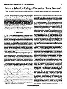
been further improved if additional samples of the genuine class were available in the training set. The ROC curves for the different discriminant approaches presented in this paper are pictorially depicted in Figure 1. The ROC curves have been calculated in the test set of the Configuration I. The best performance has been achieved when an initial PCA step was used prior to discriminant analysis. MEGM is an acronym for the modified morphological elastic graph matching using no discriminant features. MEGM-F is a notation for MEGM when the one dimension discriminant transform of the criterion in (9) was used. MEGM-D is used as a notation for the MEGM with the three most discriminant features of the multidimensional LDA. The depicted ROC curves illustrate that the performance of the EGM algorithm is highly improved by using proper linear discriminant analysis algorithms.

Figure 1: ROC curves for the different discriminant variants of NMEGM in test set of the Configuration I experimental protocol of the XM2VTS database. 5. CONCLUSIONS The use of linear discriminant techniques in the feature vectors of the elastic graph has been investigated for frontal face verification. One dimensional and multidimensional linear projections have been used in order to form the discriminant transforms for a two class problem. All experiments have been conducted in XM2VTS where a major improvement in performance has been achieved. REFERENCES [1] M. Lades, J. C. Vorbr¨uggen, J. Buhmann, J. Lange, C. v. d. Malsburg, R. P. W¨urtz, and W. Konen, “Distortion invariant object recognition in the dynamic link architecture,” IEEE Transactions on Computers, vol. 42, no. 3, pp. 300–311, Mar. 1993. [2] B. Duc, S. Fischer, and J. Big¨un, “Face authentication with Gabor information on deformable graphs,” IEEE Transactions on Image Processing, vol. 8, no. 4, pp. 504–516, Apr. 1999. [3] C. Kotropoulos, A. Tefas, and I. Pitas, “Frontal face authentication using discriminating grids with morphological feature vectors.,” IEEE Transactions on Multimedia, vol. 2, no. 1, pp. 14–26, Mar. 2000. [4] A. Tefas, C. Kotropoulos, and I. Pitas, “Using support vector machines to enhance the performance of elastic graph matching for frontal face authentication,” IEEE Transactions on Pattern Analysis and Machine Intelligence, vol. 23, no. 7, pp. 735–746, 2001.

[5] K. Fukunaga, Statistical Pattern Recognition, CA: Academic, San Diego, 1990. [6] C. Songcan and Y. Xubing, “Alternative linear discriminant classifier,” Pattern Recognition, vol. 37, no. 7, pp. 1545–1547, 2004. [7] H. Yu and J. Yang, “A direct lda algorithm for highdimensional data with application to face recognition,” Pattern Recognition, vol. 34, pp. 2067–2070, 2001. [8] D. L. Swets and J. Weng, “Using discriminant eigenfeatures for image retrieval,” IEEE Transactions on Pattern Analysis and Machine Intelligence, vol. 18, no. 8, pp. 831–836, 1996. [9] L. Juwei, K.N. Plataniotis, and A.N. Venetsanopoulos, “Face recognition using lda-based algorithms,” IEEE Transactions on Neural Networks, vol. 14, no. 1, pp. 195–200, 2003. [10] L. Juwei, K.N. Plataniotis, and A.N. Venetsanopoulos, “Face recognition using kernel direct discriminant analysis algorithms,” IEEE Transactions on Neural Networks, vol. 14, no. 1, pp. 117–126, 2003. [11] K. Messer, J. Matas, J.V. Kittler, J. Luettin, and G. Maitre, “Xm2vtsdb: The extended m2vts database,” in Proc. Second International Conf. on Audio- and Video-based Biometric Person Authentication (AVBPA’99), 1999, pp. 72–77. [12] K. Jonsson, J. Matas, and Kittler, “Learning salient features for real-time face verification,” in Proc. Second International Conf. on Audio- and Video-based Biometric Person Authentication (AVBPA’99), 1999, pp. 60–65.