LINEAR PROGRAMMING RELAXATIONS OF QUADRATICALLY CONSTRAINED QUADRATIC PROGRAMS ANDREA QUALIZZA1 , PIETRO BELOTTI2 , AND FRANC ¸ OIS MARGOT1,3 Abstract. We investigate the use of linear programming tools for solving semidefinite programming relaxations of quadratically constrained quadratic problems. Classes of valid linear inequalities are presented, including sparse P SD cuts, and principal minors P SD cuts. Computational results based on instances from the literature are presented. Key words. Quadratic Programming, Semidefinite Programming, relaxation, Linear Programming. AMS(MOS) subject classifications. 90C57
1. Introduction. Many combinatorial problems have Linear Programming (LP) relaxations that are commonly used for their solution through branch-and-cut algorithms. Some of them also have stronger relaxations involving positive semidefinite (P SD) constraints. In general, stronger relaxations should be preferred when solving a problem, thus using these P SD relaxations is tempting. However, they come with the drawback of requiring a Semidefinite Programming (SDP) solver, creating practical difficulties for an efficient implementation within a branch-and-cut algorithm. Indeed, a major weakness of current SDP solvers compared to LP solvers is their lack of efficient warm starting mechanisms. Another weakness is solving problems involving a mix of P SD constraints and a large number of linear inequalities, as these linear inequalities put a heavy toll on the linear algebra steps required during the solution process. In this paper, we investigate LP relaxations of P SD constraints with the aim of capturing most of the strength of the P SD relaxation, while still being able to use an LP solver. The LP relaxation we obtain is an outerapproximation of the P SD cone, with the typical convergence difficulties when aiming to solve problems to optimality. We thus do not cast this work as an efficient way to solve P SD problems, but we aim at finding practical ways to approximate P SD constraints with linear ones. We restrict our experiments to Quadratically Constrained Quadratic Program (QCQP). A QCQP problem with variables x ∈ Rn and y ∈ Rm is 1 Tepper
School of Business, Carnegie Mellon University, Pittsburgh PA. of Industrial and Systems Engineering, Lehigh University, Bethlehem PA. 3 Corresponding author (email:
[email protected]). Supported by NSF grant NSF-0750826. 2 Dept.
1
2
ANDREA QUALIZZA ET AL.
a problem of the form max s.t.
xT Q0 x + aT0 x + bT0 y xT Qk x + aTk x + bTk y lxi ≤ xi ≤ uxi ly j ≤ y j ≤ u y j
≤ ck
for k = 1, 2, . . . , p for i = 1, 2, . . . , n for j = 1, 2, . . . , m
(QCQP)
where, for k = 0, 1, 2, . . . , p, Qk is a rational symmetric n × n-matrix, ak is a rational n-vector, bk is a rational m-vector, and ck ∈ Q. Moreover, the lower and upper bounds lxi , uxi for i = 1, . . . , n, and lyj , uyj for j = 1, . . . , m are all finite. If Q0 is negative semidefinite and Qk is positive semidefinite for each k = 1, 2, . . . , p, problem QCQP is convex and thus easy to solve. Otherwise, the problem is NP-hard [6]. An alternative lifted formulation for QCQP is obtained by replacing each quadratic term xi xj with a new variable Xij . Let X = xxT be the matrix with entry Xij corresponding to the quadratic term xi xj . For square matrices A and B of the same dimension, let A • B denote the Frobenius inner product of A and B, i.e., the trace of AT B. Problem QCQP is then equivalent to max s.t.
Q0 • X + aT0 x + bT0 y Qk • X + aTk x + bTk y lxi ≤ xi ≤ uxi ly j ≤ y j ≤ u y j X = xxT .
≤ ck
for k = 1, 2, . . . , p for i = 1, 2, . . . , n for j = 1, 2, . . . , m
(LIFT)
The difficulty in solving problem LIFT lies in the non-convex constraint X = xxT . A relaxation, dubbed P SD, that is possible to solve relatively efficiently is obtained by relaxing this constraint to the requirement that X − xxT be positive semidefinite, i.e., X − xxT º 0. An alternative relaxation of QCQP, dubbed RLT , is obtained by the Reformulation Linearization Technique [17], using products of pairs of original constraints and bounds and replacing nonlinear terms with new variables. Anstreicher [2] compares the P SD and RLT relaxations on a set of quadratic problems with box constraints, i.e., QCQP problems with p = 0 and with all the variables bounded between 0 and 1. He shows that the P SD relaxations of these instances are fairly good and that combining the P SD and RLT relaxations yields significantly tighter relaxations than either of the P SD or RLT relaxations. The drawback of combining the two relaxations is that current SDP solvers have difficulties to handle the large number of linear constraints of the RLT . Our aim is to solve relaxations of QCQP using exclusively linear programming tools. The RLT is readily applicable for our purposes, while the P SD technique requires a cutting plane approach as described in Section 2.
LP RELAXATIONS OF QUADRATIC PROGRAMS
3
In Section 3 we consider several families of valid cuts. The focus is essentially on capturing the strength of the positive semidefinite condition using standard cuts [18], and some sparse versions of these. We analyze empirically the strength of the considered cuts on instances taken from GLOBALLib [10] and quadratic programs with box constraints described in more details in the next section. Implementation and computational results are presented in Section 4. Finally, Section 5 summarizes the results and gives possible directions for future research. 2. Relaxations of QCQP problems. A typical approach to get bounds on the optimal value of a QCQP is to solve a convex relaxation. Since our aim is to work with linear relaxations, the first step is to linearize LIFT by relaxing the last constraint to X = X T . We thus get the Extended formulation max s.t.
Q0 • X + aT0 x + bT0 y Qk • X + aTk x + bTk y lxi ≤ xi ≤ uxi ly j ≤ y j ≤ u y j X = XT .
≤ ck
for k = 1, 2, . . . , p for i = 1, 2, . . . , n for j = 1, 2, . . . , m
(EXT)
EXT is a Linear Program with n(n + 3)/2 + m variables and the same number of constraints as QCQP. Note that the optimal value of EXT is usually a weak upper bound for QCQP, as no constraint links the values of the x and X variables. Two main approaches for doing that have been proposed and are based on relaxations of the last constraint of LIFT, namely X − xxT = 0.
(2.1)
They are known as the Positive Semidefinite (P SD) relaxation and the Reformulation Linearization Technique (RLT ) relaxation. 2.1. PSD Relaxation. As X − xxT = 0 implies X − xxT < 0, using this last constraint yields a convex relaxation of QCQP. This is the approach used in [18, 20, 21, 23], among others. Moreover, using Schur’s complement X − xxT < 0
⇔
µ
1 xT x X
< 0,
and defining ˜k = Q
µ
−ck ak /2
¶ aTk /2 , Qk
˜= X
1 xT x X
µ
,
4
ANDREA QUALIZZA ET AL.
we can write the P SD relaxation of QCQP in the compact form max s.t.
˜0 • X ˜ + bT y Q 0 ˜•X ˜ + bT y ≤ 0 Q k lxi ≤ xi ≤ uxi ly j ≤ y j ≤ u y j ˜ < 0. X
k = 1, 2, . . . , p i = 1, 2, . . . , n j = 1, 2, . . . , m
(PSD)
This is a positive semidefinite problem with linear constraints. It can thus be solved in polynomial time using interior point algorithms. PSD is tighter than usual linear relaxations for problems such as the Maximum Cut, Stable Set, and Quadratic Assignment problems [25]. All these problems can be formulated as QCQPs. 2.2. RLT Relaxation. The Reformulation Linearization Technique [17] can be used to produce a relaxation of QCQP. It adds linear inequalities to EXT. These inequalities are derived from the variable bounds and constraints of the original problem as follows: multiply together two original constraints or bounds and replace each product term xi xj with the variable Xij . For instance, let xi , xj , i, j ∈ {1, 2, . . . , n} be two variables from QCQP. By taking into account only the four original bounds xi − lxi ≥ 0, xi − uxi ≤ 0, xj − lxj ≥ 0, xj − uxj ≤ 0, we get the RLT inequalities Xij Xij Xij Xij
− lxi xj − lxj xi − uxi xj − uxj xi − lxi xj − uxj xi − uxi xj − lxj xi
≥ −lxi lxj , ≥ −uxi uxj , ≤ −lxi uxj , ≤ −uxi lxj .
(2.2)
Anstreicher [2] observes that, for Quadratic Programs with box constraints, the P SD and RLT constraints together yield much better bounds than those obtained from the PSD or RLT relaxations. In this work, we want to capture the strength of both techniques and generate a Linear Programming relaxation of QCQP. Notice that the four inequalities above, introduced by McCormick [12], constitute the convex envelope of the set {(xi , xj , Xij ) ∈ R3 : lxi ≤ xi ≤ uxi , lxj ≤ xj ≤ uxj , Xij = xi xj } as proven by Al-Khayyal and Falk [1], i.e., they are the tightest relaxation for the single term Xij . 3. Our Framework. While the RLT constraints are linear in the variables in the EXT formulation and therefore can be added directly to EXT, this is not the case for the P SD constraint. We use a linear outer-approximation of the PSD relaxation and a cutting plane framework, adding a linear inequality separating the current solution from the P SD cone. The initial relaxation we use and the various cuts generated by our separation procedure are described in more details in the next sections.
5
LP RELAXATIONS OF QUADRATIC PROGRAMS
3.1. Initial Relaxation. Our initial relaxation is the EXT formulation together with the O(n2 ) RLT constraints derived from the bounds on the variables xi , i = 1, 2, . . . , n. We did not include the RLT constraints derived from the problem constraints due to their large number and the fact that we want to avoid the introduction of extra variables for the multivariate terms that occur when quadratic constraints are multiplied together. The bounds [Lij , Uij ] for the extended variables Xij are computed as follows: Lij = min{lxi lxj ; lxi uxj ; uxi lxj ; uxi uxj }, ∀i = 1, 2, . . . , n; j = i, . . . , n Uij = max{lxi lxj ; lxi uxj ; uxi lxj ; uxi uxj }, ∀i = 1, 2, . . . , n; j = i, . . . , n. In addition, equality (2.1) implies Xii ≥ x2i . We therefore also make sure that Lii ≥ 0. In the remainder of the paper, this initial relaxation is identified as EXT+RLT. 3.2. PSD Cuts. We use the equivalence that a matrix is positive semidefinite if and only if ˜ ≥0 v T Xv
for all v ∈ Rn+1 .
(3.1)
We can reformulate PSD as the semi-infinite Linear Program max s.t.
˜0 • X ˜ + bT y Q 0 ˜•X ˜ + bT y Q k lxi ≤ xi ≤ uxi ly j ≤ y j ≤ u y j ˜ v T Xv
≤ ck
≥0
for for for for
k = 1, 2, . . . , p i = 1, 2, . . . , n j = 1, 2, . . . , m all v ∈ Rn+1 .
(PSDLP)
A practical way to use PSDLP is to adopt a cutting plane approach to separate constraints (3.1) as done in [18]. ˜ ∗ be an arbitrary point in the space of the X ˜ variables. The Let X ∗ ∗ ˜ ˜ spectral decomposition of X is used to decide if X is in the P SD cone or ˜∗ not. Let the eigenvalues and corresponding orthonormal eigenvectors of X be λk and vk for k = 1, 2, . . . , n, and assume without loss of generality that λ1 ≤ λ2 ≤ . . . ≤ λn and let t ∈ {0, . . . , n} such that λt < 0 ≤ λt+1 . If t = 0, ˜ ∗ is positive semidefinite. then all the eigenvalues are non negative and X T ˜∗ T Otherwise, vk X vk = vk λk vk = λk < 0 for k = 1, . . . , t. Hence, the valid cut ˜ k≥0 vkT Xv
(3.2)
˜ ∗ . Cuts of the form (3.2) are called PSDCUTs in the is violated by X remainder of the paper. The above procedure has two major weaknesses: First, only one cut is obtained from eigenvector vk for k = 1, . . . , t, while computing the spectral
6
ANDREA QUALIZZA ET AL.
˜ pctN Z , pctV IOL ) Sparsify(v, X, ˜ · pctV IOL 1 minVIOL ← −v T Xv 2 maxNZ ← ⌊length[v] · pctN Z ⌋ 3 w←v 4 perm ← random permutation of 1 to length[w] 5 for j ← 1 to length[w] 6 do 7 z ← w, z[perm[j]] ← 0 ˜ > minV IOL 8 if −z T Xz 9 then w ← z 10 if number of non-zeroes in w < maxN Z 11 then output w Fig. 1. Sparsification procedure for PSD cuts
decomposition requires a non trivial investment in cpu time, and second, the cuts are usually very dense, i.e. almost all entries in vv T are nonzero. Dense cuts are frowned upon when used in a cutting plane approach, as they might slow down considerably the reoptimization of the linear relaxation. To address these weaknesses, we describe in the next section a heuristic to generate several sparser cuts from each of the vectors vk for k = 1, . . . , t. 3.3. Sparsification of PSD cuts. A simple idea to get sparse cuts is to start with vector w = vk , for k = 1, . . . , t, and iteratively set to zero ˜ ∗ w remains sufficiently negative. some component of w, provided that wT X If the entries are considered in random order, several cuts can be obtained from a single eigenvector vk . For example, consider the Sparsify procedure ˜ and two in Figure 1, taking as parameters an initial vector v, a matrix X, numbers between 0 and 1, pctN Z and pctV IOL , that control the maximum percentage of nonzero entries in the final vector and the minimum violation requested for the corresponding cut, respectively. In the procedure, parameter length[v] identifies the size of vector v. It is possible to implement this procedure to run in O(n2 ) if length[v] = n + 1: Compute and update a vector m such that mj =
n+1 X
˜ ij for j = 1, . . . , n + 1 . wj wi X
i=1
Its initial computation takes O(n2 ) and its update, after a single entry of w is set to 0, takes O(n). The vector m can be used to compute the left hand side of the test in step 8 in constant time given the value of the violation d for the inequality generated by the current vector w: Setting the entry ˜ ℓℓ and thus ℓ = perm[j] of w to zero reduces the violation by 2mℓ − wℓ2 X 2 ˜ the violation of the resulting vector is (d − 2mℓ + wℓ Xℓℓ ).
LP RELAXATIONS OF QUADRATIC PROGRAMS
7
A slight modification of the procedure is used to obtain several cuts from the same eigenvector: Change the loop condition in step 5 to consider the entries in perm in cyclical order, from all possible starting points s in {1, 2 . . . , length[w]}, with the additional condition that entry s − 1 is not set to 0 when starting from s to guarantee that we do not generate always the same cut. From our experiments, this simple idea produces collections of sparse and well-diversified cuts. This is referred to as SPARSE1 in the remainder of the paper. We also consider the following variant of the procedure given in Fig˜ [w] be the principal minor of X ˜ induced by ure 1. Given a vector w, let X the indices of the nonzero entries in w. Replace step 7 with 7. z ← w ¯ where w ¯ is an eigenvector corresponding to the most negative eigenvalue of a spectral decomposition of ˜ [w] , z[perm[j]] ← 0. X This is referred to as SPARSE2 in the remainder, and we call the cuts generated by SPARSE1 or SPARSE2 described above Sparse P SD cuts. Once sparse P SD cuts are generated, for each vector w generated, we can also add all P SD cuts given by the eigenvectors corresponding to ˜ [w] . These cuts are negative eigenvalues of a spectral decomposition of X valid and sparse. They are called Minor P SD cuts and denoted by MINOR in the following. An experiment to determine good values for the parameters pctN Z and pctV IOL was performed on the 38 GLOBALLIB instances and 51 BoxQP instances described in Section 4.1. It is run by selecting two sets of three values in [0, 1], {VLOW , VM ID , VU P } for pctV IOL and {NLOW , NM ID , NU P } for pctN Z . The nine possible combinations of these parameter values are used and the best of the nine (Vbest , Nbest ) is selected. We then center and reduce the possible ranges around Vbest and Nbest , respectively, and repeat the operation. The procedure is stopped when the best candidate parameters are (VM ID , NM ID ) and the size of the ranges satisfy |VU P − VLOW | ≤ 0.2 and |NU P − NLOW | ≤ 0.1. In order to select the best value of the parameters, we compare the bounds obtained by both algorithms after 1, 2, 5, 10, 20, and 30 seconds of computation. At each of these times, we count the number of times each algorithm outperforms the other by at least 1% and the winner is the algorithm with the largest number of wins over the 6 clocked times. It is worth noting that typically the majority of the comparisons end up as ties, implying that the results are not extremely sensitive to the selected values for the parameters. For SPARSE1, the best parameter values are pctV IOL = 0.6 and pctN Z = 0.2. For SPARSE2, they are pctV IOL = 0.6 and pctN Z = 0.4. These values are used in all experiments using either SPARSE1 or SPARSE2 in the remainder of the paper.
8
ANDREA QUALIZZA ET AL.
4. Computational Results. In the implementation, we have used the Open Solver Interface (Osi-0.97.1) from COIN-OR [8] to create and modify the LPs and to interface with the LP solvers ILOG Cplex-11.1. To compute eigenvalues and eigenvectors, we use the dsyevx function provided by the LAPACK library version 3.1.1. We also include a cut management procedure to reduce the number of constraints in the outer approximation LP. This procedure, applied at the end of each iteration, removes the cuts that are not satisfied with equality by the optimal solution. Note however that the constraints from the EXT+RLT formulation are never removed, only constraints from added cutting planes are possibly removed. The machine used for the tests is a 64 bit 2.66GHz AMD processor, 64GB of RAM memory, and Linux kernel 2.6.29. Tolerances on the accuracy of the primal and dual solutions of the LP solver and LAPACK calls are set to 10−8 . The set of instances used for most experiments consists of 51 BoxQP instances with at most 50 variables and the 38 GLOBALLib instances as described in Section 4.1. For an instance I and a given relaxation of it, we define the gap closed by the relaxation as 100 ·
RLT − BN D , RLT − OP T
(4.1)
where BN D and RLT are the optimal value for the given relaxation and the EXT+RLT relaxation respectively, and OP T is either the optimal value of I or the best known value for a feasible solution. The OP T values are taken from [14]. 4.1. Instances. Tests are performed on a subset of instances from GLOBALLib [10] and on Box Constrained Quadratic Programs (BoxQPs) [24]. GLOBALLib contains 413 continuous global optimization problems of various sizes and types, such as BoxQPs, problems with complementarity constraints, and general QCQPs. Following [14], we select 160 instances from GLOBALLib having at most 50 variables and that can easily be formulated as QCQP. The conversion of a non-linear expression into a quadratic expression, when possible, is performed by adding new variables and constraints to the problem. Additionally, bounds on the variables are derived using linear programming techniques and these bound are included in the formulation. From these 160 instances in AMPL format, we substitute each bilinear term xi xj by the new variable Xij as described for the LIFT formulation. We build two collections of linearized instances in MPS format, one with the original precision on the coefficients and right hand side, and the second with 8-digit precision. In our experiments we used the latter. As observed in [14], using together the SDP and RLT relaxations yields stronger bounds than those given by the RLT relaxation only for 38
LP RELAXATIONS OF QUADRATIC PROGRAMS
9
out of 160 GLOBALLib instances. Hence, we focus on these 38 instances to test the effectiveness of the P SD Cuts and their sparse versions. The BoxQP collection contains 90 instances with a number of variables ranging from 20 to 100. Due to time limit constraints and the number of experiments to run, we consider only instances with a number of variables between 20 to 50, for a total of 51 BoxQP problems. The converted GLOBALLib and BoxQP instances are available in MPS format from [13]. 4.2. Effectiveness of each class of cuts. We first compare the effectiveness of the various classes of cuts when used in combination with the standard PSDCUTs. For these tests, at most 1,000 cutting iterations are performed, at most 600 seconds are used, and operations are stopped if tailing off is detected. More precisely, let zt be the optimal value of the linear relaxation at iteration t. The operations are halted if t ≥ 50 and zt ≥ (1 − 0.0001) · zt−50 . A cut purging procedure is used to remove cuts that are not tight at iteration t if the condition zt ≥ (1 − 0.0001) · zt−1 is 2 satisfied. On average in each iteration the algorithm generates n2 cuts, of which only n2 are are kept by the cut purging procedure and the rest are discarded. In order to compare two different cutting plane algorithms, we compare the closed gaps values first after a fixed number of iterations, and second at several given times, for all QCQP instances at avail. Comparisons at fixed iterations indicate the quality of the cuts, irrespective of the time used to generate them. Comparisons at given times are useful if only limited time is available for running the cutting plane algorithms and a good approximation of the P SD cone is sought. The closed gaps obtained at a given point are deemed different only if their difference is at least g% of the initial gap. We report comparisons for g = 1 and g = 5. Comparisons at one point is possible only if both algorithms reach that point. The number of problems for which this does not happen – because, at a given time, either result was not available or one of the two algorithms had already stopped, or because either algorithm had terminated in fewer iterations – is listed in the “inc.” (incomparable) columns in the tables. For the remaining problems, we report the percentage of problems for which one algorithm is better than the other and the percentage of problems were they are tied. Finally, we also report the average improvement in gap closed for the second algorithm over the first algorithm in the column labeled “impr.”. Tests are first performed to decide which combination of the SPARSE1, SPARSE2 and MINOR cuts perform best on average. Based on Tables 1 and 2 below, we conclude that using MINOR is useful both in terms of iteration and time, and that the algorithm using PSDCUT+SPARSE2+MINOR (abbreviated S2M in the remainder) dominates the algorithm using PSDCUT+SPARSE1+MINOR (abbreviated S1M) both in terms of iteration and time. Table 1 gives the comparison between S1M and S2M at differ-
10
ANDREA QUALIZZA ET AL.
ent iterations. S2M dominates clearly S1M in the very first iteration and after 200 iterations, while after the first few iterations S1M also manages to obtain good bounds. Table 2 gives the comparison between these two algorithms at different times. For comparisons with g = 1, S1M is better than S2M only in at most 2.25% of the problems, while the converse varies between roughly 50% (at early times) and 8% (for late times). For g = 5, S2M still dominates S1M in most cases. Table 1 Comparison of S1M with S2M at several iterations.
g=1
g=5
Iteration
S1M
S2M
Tie
S1M
S2M
Tie
inc.
impr.
1 2 3 5 10 15 20 30 50 100 200 300 500 1000
7.87 17.98 17.98 12.36 10.11 4.49 1.12 1.12 2.25 0.00 0.00 0.00 0.00 0.00
39.33 28.09 19.10 14.61 13.48 13.48 10.11 8.99 6.74 4.49 3.37 2.25 2.25 2.25
52.80 53.93 62.92 73.03 76.41 82.03 78.66 79.78 80.90 28.09 15.73 12.36 7.87 3.37
1.12 0.00 1.12 3.37 0.00 1.12 1.12 1.12 1.12 0.00 0.00 0.00 0.00 0.00
19.1 10.11 7.87 5.62 5.62 6.74 6.74 5.62 4.49 2.25 2.25 2.25 2.25 2.25
79.78 89.89 91.01 91.01 94.38 92.14 82.02 83.15 84.28 30.33 16.85 12.36 7.87 3.37
0.00 0.00 0.00 0.00 0.00 0.00 10.11 10.11 10.11 67.42 80.90 85.39 89.88 94.38
3.21 2.05 1.50 1.77 1.42 1.12 1.02 0.79 0.47 1.88 2.51 3.30 3.85 7.43
Sparse cuts yield better bounds than using solely the standard P SD cuts. The observed improvement is around 3% and 5% respectively for SPARSE1 and SPARSE2. When we are using the MINOR cuts, this value gets to 6% and 8% respectively for each type of sparsification algorithm used. Table 3 compares PSDCUT (abbreviated by S) with S2M. The table shows that the sparse cuts generated by the sparsification procedures and minor P SD cuts yield better bounds than the standard cutting plane algorithm at fixed iterations. Comparisons performed at fixed times, on the other hand, show that considering the whole set of instances we do not get any improvement in the first 60 to 120 seconds of computation (see Table 4). Indeed S2M initially performs worse than the standard cutting plane algorithm, but after 60 to 120 seconds, it produces better bounds on average. In Section 6 detailed computational results are given in Tables 5 and 6 where for each instance we compare the duality gap closed by S and S2M at several iterations and times. The initial duality gap is obtained as in (4.1) as RLT − OP T . We then let S2M run with no time limit until the
11
LP RELAXATIONS OF QUADRATIC PROGRAMS Table 2 Comparison of S1M with S2M at several times.
g=1
g=5
Time
S1M
S2M
Tie
S1M
S2M
Tie
inc.
impr.
0.5 1 2 3 5 10 15 20 30 60 120 180 300 600
3.37 0.00 0.00 1.12 1.12 1.12 2.25 1.12 1.12 1.12 0.00 0.00 0.00 0.00
52.81 51.68 47.19 44.94 43.82 41.58 37.08 35.96 28.09 20.23 15.73 13.49 11.24 7.86
12.36 14.61 15.73 14.61 15.73 16.85 16.85 16.85 22.48 28.09 32.58 32.58 31.46 24.72
0.00 0.00 0.00 0.00 0.00 0.00 1.12 1.12 1.12 0.00 0.00 0.00 0.00 0.00
43.82 40.45 39.33 34.83 38.20 24.72 21.35 17.98 16.86 12.36 10.11 5.62 3.37 0.00
24.72 25.84 23.59 25.84 22.47 34.83 33.71 34.83 33.71 37.08 38.20 40.45 39.33 32.58
31.46 33.71 37.08 39.33 39.33 40.45 43.82 46.07 48.31 50.56 51.69 53.93 57.30 67.42
2.77 4.35 5.89 5.11 6.07 4.97 3.64 3.49 2.99 2.62 1.73 1.19 0.92 0.72
Table 3 Comparison of S with S2M at several iterations.
g=1
g=5
Iteration
S
S2M
Tie
S
S2M
Tie
inc.
impr.
1 2 3 5 10 15 20 30 50 100 200 300 500 1000
0.00 0.00 0.00 0.00 1.12 1.12 1.12 1.12 1.12 1.12 0.00 0.00 0.00 0.00
76.40 84.27 83.15 80.90 71.91 60.67 53.93 34.83 25.84 8.99 5.62 3.37 3.37 2.25
23.60 15.73 16.85 19.10 26.97 38.21 40.45 53.93 62.92 21.35 8.99 7.87 5.62 0.00
0.00 0.00 0.00 0.00 0.00 1.12 1.12 0.00 0.00 0.00 0.00 0.00 0.00 0.00
61.80 55.06 48.31 40.45 41.57 35.96 29.21 16.85 13.48 5.62 3.37 3.37 3.37 2.25
38.20 44.94 51.69 59.55 58.43 62.92 65.17 73.03 76.40 25.84 11.24 7.87 5.62 0.00
0.00 0.00 0.00 0.00 0.00 0.00 4.50 10.12 10.12 68.54 85.39 88.76 91.01 97.75
10.47 10.26 10.38 10.09 8.87 7.49 6.22 5.04 3.75 5.57 7.66 8.86 8.72 26.00
value s obtained does not improve by at least 0.01% over ten consecutive iterations. This value s is an upper bound on the value of the PSD+RLT relaxation. The column “bound” in the tables gives the value of RLT − s as a percentage of the gap RLT − OP T , i.e. an approximation of the percentage of the gap closed by the PSD+RLT relaxation. The columns
12
ANDREA QUALIZZA ET AL. Table 4 Comparison of S with S2M at several times.
g=1
g=5
Time
S
S2M
Tie
S
S2M
Tie
inc.
impr.
0.5 1 2 3 5 10 15 20 30 60 120 180 300 600
41.57 41.57 42.70 41.57 35.96 34.84 37.07 37.07 30.34 11.24 8.99 2.25 0.00 0.00
17.98 14.61 10.11 8.99 7.87 7.87 5.62 5.62 5.62 12.36 12.36 14.61 15.73 14.61
5.62 5.62 6.74 8.99 15.72 13.48 11.24 8.99 15.72 25.84 24.72 29.21 26.97 13.48
41.57 39.33 29.21 31.46 33.71 30.34 22.47 17.98 11.24 11.24 2.25 0.00 0.00 0.00
17.98 13.48 8.99 6.74 5.62 4.50 2.25 1.12 1.12 2.25 2.25 4.50 6.74 5.62
5.62 8.99 21.35 21.35 20.22 21.35 29.21 32.58 39.32 35.95 41.57 41.57 35.96 22.47
34.83 38.20 40.45 40.45 40.45 43.81 46.07 48.32 48.32 50.56 53.93 53.93 57.30 71.91
-9.42 -8.66 -8.73 -8.78 -7.87 -5.95 -5.48 -4.99 -3.9 -1.15 0.48 1.09 1.60 2.73
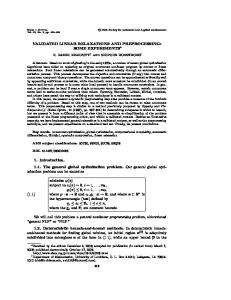
labeled S and S2M in the tables give the gap closed by the corresponding algorithms at different iterations. Note that although S2M relies on numerous spectral decomposition computations, most of its running time is spent in generating cuts and reoptimization of the LP. For example, on the BoxQP instances with a time limit of 300 seconds, the average percentage of CPU time spent for obtaining spectral decompositions is below 21 for instances of size 30, below 15 for instances of size 40 and below 7 for instances of size 50. 5. Conclusions. This paper studies linearizations of the P SD cone based on spectral decompositions. Sparsification of eigenvectors corresponding to negative eigenvalues is shown to produce useful cuts in practice, in particular when the minor cuts are used. The goal of capturing most of the strength of an P SD relaxation through linear inequalities is achieved, although tailing off occurs relatively quickly. As an illustration of typical behavior of a P SD solver and our linear outer-approximation scheme, consider the two instances, spar020-100-1 and spar030-060-1, with respectively 20 and 30 variables. We use the SDP solver SeDuMi and S2M, keeping track at each iteration of the bound achieved and the time spent. Figure 2 and Figure 3 compare the bounds obtained by the two solvers at a given time. For the small size instance spar020-100-1, we note that S2M converges to the bound value more than twenty times faster than SeDuMi. In the medium size instance spar030-060-1 we note that S2M closes a large gap in the first ten to twenty iterations, and then tailing off occurs. To compute the exact bound, SeDuMi requires 408 seconds while S2M requires 2,442
13
LP RELAXATIONS OF QUADRATIC PROGRAMS
seconds to reach the same precision. Nevertheless, for our purposes, most of the benefits of the P SD constraints are captured in the early iterations. Two additional improvements are possible. The first one is to use a cut separation procedure for the RLT inequalities, avoiding their inclusion in the initial LP and managing them as other cutting planes. This could potentially speed up the reoptimization of the LP. Another possibility is to use a mix of the S and S2M algorithms, using the former in the early iterations and then switching to the latter. Fig. 2. Instance spar020-100-1 750
700
Bound
650 SeDuMi S2M
600 bound
550
500 0
5
10
15
20
25
30
35
40
Time (s)
Fig. 3. Instance spar030-060-1 1250
1150
1050
Bound
950 SeDuMi S2M
850
bound
750
650
550 0
50
100
150
200
250
300
350
400
450
Time (s)
Acknowledgments. The authors warmly thank Anureet Saxena for the useful discussions that led to the results obtained in this work.
14
6. Appendix. Table 5 Duality gap closed at several iterations for each instance.
Instance
|x|
|y|
45.79 100.00 22.05 49.75 100.00 56.40 100.00 100.00 100.00 100.00 100.00 68.26 77.43 91.81 54.52 70.37 99.87 99.88 42.30 49.75 52.06 100.00 100.00 100.00 53.97 100.00 100.00 8.00
iter. 2 S S2M 0.00 25.59 3.93 49.75 99.81 0.00 22.33 69.44 18.00 56.90 94.91 32.32 3.04 4.45 0.00 0.00 0.00 3.50 0.00 49.75 0.00 95.76 99.84 0.00 26.00 90.61 0.00 0.00
0.00 27.92 8.65 49.75 99.84 0.00 42.78 69.87 48.17 81.93 95.19 39.17 33.75 21.80 42.55 14.08 24.84 99.42 4.59 49.75 20.87 100.00 99.93 0.00 26.41 92.39 99.00 4.25
iter. 10 S S2M 10.97 37.25 15.93 49.75 100.00 51.19 98.98 92.62 96.86 99.76 99.98 59.01 33.13 18.60 0.01 2.34 25.24 23.09 0.00 49.75 21.95 99.96 100.00 78.35 48.49 98.39 61.14 0.00
41.31 35.76 21.05 49.75 100.00 51.19 99.98 99.94 99.90 99.93 100.00 66.76 53.44 45.08 50.13 51.97 99.85 99.86 27.34 49.75 29.03 100.00 100.00 95.84 50.16 98.39 99.96 4.98
iter. 50 S S2M 45.77 95.90 22.05 49.75 100.00 56.40 100.00 100.00 100.00 100.00 100.00 68.00 64.03 38.07 0.01 7.12 86.37 62.32 3.14 49.75 26.04 100.00 100.00 100.00 53.87 98.39 99.64 0.00
45.79 92.17 22.05 49.75 100.00 56.40 100.00 100.00 100.00 100.00 100.00 68.25 75.38 69.83 51.90 69.41 99.87 99.88 34.91 49.75 31.39 100.00 100.00 100.00 53.96 98.39 100.00 5.73
ANDREA QUALIZZA ET AL.
circle 3 0 dispatch 3 1 20 0 ex2 1 10 ex3 1 2 5 0 ex4 1 1 3 0 3 0 ex4 1 3 ex4 1 4 3 0 3 0 ex4 1 6 ex4 1 7 3 0 3 0 ex4 1 8 ex8 1 4 4 0 ex8 1 5 5 0 9 0 ex8 1 7 ex8 4 1 21 1 10 0 ex9 2 1 ex9 2 2 10 0 6 2 ex9 2 4 ex9 2 6 16 0 ex9 2 7 10 0 5 4 himmel11 hydro 12 19 4 0 mathopt1 mathopt2 3 0 meanvar 7 1 5 0 nemhaus prob06 2 0 3 1 prob09 process 9 3 Continued on Next Page. . .
bound
Table 5 – Continued Instance
|x|
|y|
100.00 100.00 100.00 100.00 100.00 93.51 87.55 49.75 97.99 97.93 100.00 99.70 100.00 98.87 100.00 99.40 97.99 100.00 99.98 98.99 100.00 100.00 100.00 100.00 100.00 100.00 99.96 99.85 100.00 100.00 100.00 96.74 100.00 99.18 99.42
iter. 2 S S2M 79.59 55.94 97.48 56.90 0.00 5.14 55.80 49.75 71.99 70.55 91.15 90.12 96.96 43.53 80.74 67.43 49.05 81.19 85.97 64.44 92.78 92.71 80.37 86.09 90.65 77.28 76.78 86.82 25.60 30.93 9.21 23.62 33.17 21.77 35.62
89.09 70.99 100.00 81.93 0.00 15.93 55.80 49.75 76.69 75.16 94.64 92.64 98.51 53.64 89.73 71.94 54.94 85.82 87.43 70.99 95.45 94.18 86.35 89.26 91.56 83.25 81.65 88.74 41.96 53.39 31.38 29.03 48.87 30.31 44.87
iter. 10 S S2M 93.89 82.42 99.96 99.76 98.72 29.97 87.02 49.75 97.20 94.93 99.77 98.17 100.00 79.61 99.89 91.48 76.54 99.26 98.44 87.32 100.00 99.99 97.27 98.13 99.97 95.20 93.44 97.45 73.59 79.34 66.46 63.04 89.08 70.44 73.11
99.77 93.92 100.00 99.93 98.72 60.10 87.01 49.75 97.95 97.52 99.99 99.32 100.00 87.39 100.00 95.68 86.51 99.99 99.52 92.11 100.00 100.00 99.30 99.65 100.00 98.30 96.84 98.75 84.72 95.62 86.62 75.93 97.94 80.96 84.05
iter. 50 S S2M 98.93 93.04 100.00 100.00 100.00 93.40 87.23 49.75 97.99 97.93 100.00 99.66 100.00 93.90 100.00 98.75 91.15 100.00 99.92 96.23 100.00 100.00 100.00 100.00 100.00 99.85 98.70 99.75 99.13 99.46 98.53 85.93 100.00 91.37 92.81
100.00 99.35 100.00 100.00 100.00 93.50 87.23 49.75 97.99 97.93 100.00 99.69 100.00 97.14 100.00 99.26 95.68 100.00 99.97 98.01 100.00 100.00 100.00 100.00 100.00 100.00 99.72 99.83 100.00 100.00 100.00 93.29 100.00 96.69 97.21
LP RELAXATIONS OF QUADRATIC PROGRAMS
15
qp1 50 0 50 0 qp2 rbrock 3 0 st e10 3 1 2 0 st e18 st e19 3 1 4 0 st e25 st e28 5 4 st iqpbk1 8 0 8 0 st iqpbk2 spar020-100-1 20 0 20 0 spar020-100-2 spar020-100-3 20 0 30 0 spar030-060-1 spar030-060-2 30 0 spar030-060-3 30 0 30 0 spar030-070-1 spar030-070-2 30 0 30 0 spar030-070-3 spar030-080-1 30 0 30 0 spar030-080-2 spar030-080-3 30 0 spar030-090-1 30 0 30 0 spar030-090-2 spar030-090-3 30 0 30 0 spar030-100-1 spar030-100-2 30 0 spar030-100-3 30 0 40 0 spar040-030-1 spar040-030-2 40 0 40 0 spar040-030-3 spar040-040-1 40 0 40 0 spar040-040-2 spar040-040-3 40 0 spar040-050-1 40 0 Continued on Next Page. . .
bound
16
Table 5 – Continued |x|
|y|
bound
spar040-050-2 spar040-050-3 spar040-060-1 spar040-060-2 spar040-060-3 spar040-070-1 spar040-070-2 spar040-070-3 spar040-080-1 spar040-080-2 spar040-080-3 spar040-090-1 spar040-090-2 spar040-090-3 spar040-100-1 spar040-100-2 spar040-100-3 spar050-030-1 spar050-030-2 spar050-030-3 spar050-040-1 spar050-040-2 spar050-040-3 spar050-050-1 spar050-050-2 spar050-050-3 Average
40 40 40 40 40 40 40 40 40 40 40 40 40 40 40 40 40 50 50 50 50 50 50 50 50 50 -
0 0 0 0 0 0 0 0 0 0 0 0 0 0 0 0 0 0 0 0 0 0 0 0 0 0 -
99.48 100.00 98.09 100.00 100.00 100.00 100.00 100.00 100.00 100.00 99.99 100.00 99.97 100.00 100.00 99.87 98.70 100.00 99.27 99.29 100.00 99.39 100.00 93.02 98.74 98.84 -
iter. 2 S S2M 36.79 41.91 46.22 63.02 78.09 64.02 67.49 70.13 63.06 71.42 83.93 75.73 76.39 84.90 87.64 79.78 72.69 3.11 1.35 0.08 23.13 21.89 27.18 25.24 32.10 38.57 48.75
47.68 51.72 52.89 72.87 87.91 71.33 76.78 79.43 69.40 79.77 88.65 79.96 80.97 87.04 90.43 83.02 78.31 17.60 16.67 13.63 30.86 34.45 37.42 33.77 41.26 44.67 59.00
iter. 10 S S2M 82.38 84.04 81.65 94.09 99.30 93.92 95.12 95.65 91.09 94.98 97.76 95.34 95.16 98.33 98.27 94.58 90.83 58.23 51.11 50.19 72.10 71.24 83.96 61.42 77.48 80.97 75.53
91.27 90.70 87.28 97.66 99.99 97.35 97.97 97.99 95.44 97.62 98.86 97.43 96.72 99.52 99.35 96.76 93.03 79.98 70.58 67.46 81.73 81.63 91.70 68.75 83.48 85.36 84.39
iter. 50 S S2M 97.26 96.88 92.39 99.78 100.00 99.77 99.97 99.75 99.00 99.92 99.81 99.46 99.20 100.00 99.98 98.74 95.84 85.85
98.93 99.34 95.97 100.00 100.00 100.00 100.00 100.00 99.97 100.00 99.95 99.91 99.81 100.00 100.00 99.50 97.36 89.60
ANDREA QUALIZZA ET AL.
Instance
Table 6 Duality gap closed at several times for each instance. (Instances solved in less than 1 second are not shown)
1s bound
S2M
ex4 1 4 100.00 ex8 1 4 100.00 77.43 77.43 ex8 1 7 ex8 4 1 91.81 28.14 70.37 ex9 2 2 ex9 2 6 99.88 96.28 hydro 52.06 26.43 100.00 mathopt2 process 8.00 100.00 79.99 qp1 qp2 100.00 55.82 100.00 100.00 spar020-100-1 spar020-100-2 99.70 99.67 spar020-100-3 100.00 98.87 69.98 spar030-060-1 spar030-060-2 100.00 96.52 99.40 82.99 spar030-060-3 spar030-070-1 97.99 69.81 100.00 96.05 spar030-070-2 spar030-070-3 99.98 96.26 spar030-080-1 98.99 83.36 100.00 99.83 spar030-080-2 spar030-080-3 100.00 99.88 100.00 92.86 spar030-090-1 spar030-090-2 100.00 93.80 100.00 97.78 spar030-090-3 spar030-100-1 100.00 91.04 spar030-100-2 99.96 90.21 99.85 94.26 spar030-100-3 spar040-030-1 100.00 28.97 Continued on Next Page. . .
100.00 100.00 77.37 36.24 70.35 31.46 100.00 7.66 80.28 55.27 100.00 99.61 100.00 58.72 91.05 76.15 60.36 87.93 90.42 74.42 96.70 95.87 87.69 88.46 91.35 84.34 83.14 89.55 40.51
60 s S S2M 61.60 98.22 91.74 96.53 99.27 94.50 99.98 97.80 100.00 99.56 99.84 89.30
90.43 99.52 95.56 97.61 99.32 96.38 99.98 98.11 100.00 100.00 99.75 99.84 84.19
180 s S S2M 99.73 95.86 98.45 99.38 97.29 99.98 98.74 99.91 99.85 99.06
99.96 98.69 98.70 99.39 97.73 99.98 98.88 99.95 99.85 99.98
300 s S S2M 99.92 97.41 98.68 99.39 97.70 98.89 99.95 99.85 99.98
99.98 99.66 98.82 99.40 97.91 99.98 98.96 99.96 99.85 100.00
600 s S S2M 99.99 98.80 99.40 99.85 -
100.00 100.00 99.40 97.98 98.99 99.96 99.85 100.00
17
S
LP RELAXATIONS OF QUADRATIC PROGRAMS
Instance
18
Table 6 – Continued 1s bound
S
S2M
spar040-030-2 spar040-030-3 spar040-040-1 spar040-040-2 spar040-040-3 spar040-050-1 spar040-050-2 spar040-050-3 spar040-060-1 spar040-060-2 spar040-060-3 spar040-070-1 spar040-070-2 spar040-070-3 spar040-080-1 spar040-080-2 spar040-080-3 spar040-090-1 spar040-090-2 spar040-090-3 spar040-100-1 spar040-100-2 spar040-100-3 spar050-030-1 spar050-030-2 spar050-030-3 spar050-040-1 spar050-040-2 spar050-040-3 spar050-050-1 spar050-050-2 spar050-050-3 Average
100.00 100.00 96.74 100.00 99.18 99.42 99.48 100.00 98.09 100.00 100.00 100.00 100.00 100.00 100.00 100.00 99.99 100.00 99.97 100.00 100.00 99.87 98.70 100.00 99.27 99.29 100.00 99.39 100.00 93.02 98.74 98.84 -
31.97 9.20 19.38 24.51 20.88 28.96 29.52 28.67 37.16 39.57 52.41 50.01 47.57 47.22 51.66 52.24 56.05 59.71 59.14 63.07 69.47 65.27 61.40 0.37 0.08 0.00 3.76 2.08 1.76 4.91 6.18 6.12 51.45
48.01 27.59 22.90 29.87 21.31 21.27 16.91 19.81 17.10 22.83 30.57 21.79 25.19 21.95 28.00 25.94 26.98 28.17 29.82 34.62 28.24 26.07 29.61 3.63 2.79 2.75 1.77 2.84 2.31 1.84 3.39 2.82 42.96
60 s S S2M 94.01 81.66 70.35 98.63 78.28 80.18 91.33 90.03 86.26 98.09 100.00 97.74 98.81 98.96 95.13 98.71 99.54 98.10 97.83 99.94 99.66 97.34 93.01 54.46 44.68 44.32 69.97 68.64 79.44 60.64 76.56 79.38 87.50
96.39 85.43 75.45 98.60 79.31 84.01 91.42 90.72 87.13 98.22 99.99 97.78 98.46 98.70 95.38 98.31 99.25 97.86 97.70 99.85 99.47 96.87 93.17 37.52 38.62 32.31 56.87 58.47 65.71 53.28 68.33 69.23 86.38
180 s S S2M 99.58 97.25 80.73 100.00 86.02 88.70 97.01 95.68 90.18 99.90 99.80 99.99 99.88 98.29 99.95 99.89 99.43 99.34 100.00 99.99 98.60 94.91 70.10 59.58 57.13 77.15 77.72 89.73 65.52 82.34 84.95 92.14
99.98 99.86 88.63 100.00 91.22 94.62 97.97 97.51 93.50 99.96 99.87 99.99 99.92 99.05 99.97 99.88 99.61 99.58 100.00 99.99 98.98 96.02 73.34 64.94 59.07 78.30 77.61 87.74 66.42 82.21 83.23 93.22
300 s S S2M 99.99 99.81 85.34 89.52 92.75 98.26 97.49 92.25 100.00 99.97 100.00 99.98 99.09 100.00 99.94 99.70 99.68 100.00 99.02 95.81 76.87 67.79 62.54 80.31 81.54 92.67 66.81 84.94 86.99 93.18
100.00 100.00 92.29 95.04 96.71 98.87 99.08 95.32 100.00 99.99 100.00 100.00 99.74 100.00 99.95 99.86 99.81 100.00 99.39 97.00 84.75 74.98 68.99 84.30 83.63 93.00 70.38 86.52 86.98 94.77
600 s S S2M 100.00 90.79 94.07 96.53 98.92 95.05 100.00 100.00 100.00 99.77 99.97 99.90 99.86 99.44 96.84 86.23 77.02 71.18 84.90 86.40 95.99 68.45 89.77 93.16
94.74 97.71 98.32 99.31 99.89 96.84 100.00 100.00 99.99 99.98 99.99 99.93 99.69 97.77 96.33 86.58 82.86 91.79 90.94 97.69 74.76 91.34 91.57 95.86
ANDREA QUALIZZA ET AL.
Instance
LP RELAXATIONS OF QUADRATIC PROGRAMS
19
REFERENCES [1] F. A. Al-Khayyal and J. E. Falk, Jointly constrained biconvex programming. Math. Oper. Res. 8, pp. 273-286, 1983. [2] K. M. Anstreicher, Semidefinite Programming versus the Reformulation Linearization Technique for Nonconvex Quadratically Constrained Quadratic Programming. Pre-print. Optimization Online, May 2007. Available at
http://www.optimization-online.org/DB HTML/2007/05/1655.html [3] E. Balas, Disjunctive programming: properties of the convex hull of feasible points. Disc. Appl. Math. 89, 1998. [4] M. S. Bazaraa, H. D. Sherali and C. M. Shetty, Nonlinear Programming: Theory and Algorithms. Wiley, 2006. [5] S. Boyd, L. Vandenberghe, Convex Optimization. Cambridge University Press, 2004. [6] S. Burer and A. Letchford, On Non-Convex Quadratic Programming with Box Constraints. Optimization Online, July 2008. Available at
http://www.optimization-online.org/DB HTML/2008/07/2030.html [7] B. Borchers, CSDP, A C Library for Semidefinite Programming, Optimization Methods and Software 11(1), pp. 613-623, 1999. [8] COmputational INfrastructure for Operations Research (COIN-OR).
http://www.coin-or.org [9] S. J. Benson and Y. Ye, DSDP5: Software For Semidefinite Programming. Available at http://www-unix.mcs.anl.gov/DSDP [10] GamsWorld Global Optimization library.
http://www.gamsworld.org/global/globallib/globalstat.htm [11] L. Lov´ asz and A. Schrijver, Cones of matrices and set-functions and 0-1 optimization. SIAM Journal on Optimization, May 1991 [12] G.P. McCormick, Nonlinear programming: theory, algorithms and applications. John Wiley & sons, 1983. [13] http://www.andrew.cmu.edu/user/aqualizz/research/MIQCP [14] A. Saxena, P. Bonami and J. Lee, Convex Relaxations of Non-Convex Mixed Integer Quadratically Constrained Programs: Extended Formulations, 2009. To appear in Mathematical Programming. [15] , Convex Relaxations of Non-Convex Mixed Integer Quadratically Constrained Programs: Projected Formulations, Optimization Online, November 2008. Available at
http://www.optimization-online.org/DB HTML/2008/11/2145.html [16] J. F. Sturm, SeDuMi: An Optimization Package over Symmetric Cones. Available at http://sedumi.mcmaster.ca [17] H. D. Sherali and W. P. Adams, A reformulation-linearization technique for solving discrete and continuous nonconvex problems. Kluwer, Dordrecht 1998. [18] H. D. Sherali and B. M. P. Fraticelli, Enhancing RLT relaxations via a new class of semidefinite cuts. J. Global Optim. 22, pp. 233-261, 2002. [19] N.Z. Shor, Quadratic optimization problems. Tekhnicheskaya Kibernetika, 1, 1987. [20] K. Sivaramakrishnan and J. Mitchell, Semi-infinite linear programming approaches to semidefinite programming (SDP) problems. Novel Approaches to Hard Discrete Optimization, edited by P.M. Pardalos and H. Wolkowicz, Fields Institute Communications Series, American Math. Society, 2003. , Properties of a cutting plane method for semidefinite programming, Tech[21] nical Report, Department of Mathematics, North Carolina State University, September 2007. [22] K. C. Toh, M. J. Todd and R. H. T¨ ut¨ unc¨ u, SDPT3: A MATLAB software for semidefinite-quadratic-linear programming. Available at
http://www.math.nus.edu.sg/~mattohkc/sdpt3.html [23] L. Vandenberghe and S. Boyd, Semidefinite Programming. SIAM Review 38 (1), pp. 49-95, 1996.
20
ANDREA QUALIZZA ET AL.
[24] D. Vandenbussche and G. L. Nemhauser, A branch-and-cut algorithm for nonconvex quadratic programs with box constraints. Math. Prog. 102(3), pp. 559-575, 2005. [25] H. Wolkowicz, R. Saigal and L. Vandenberghe, Handbook of Semidefinite Programming: Theory, Algorithms, and Applications. Springer, 2000.