Linear Stochastic Approximation: Constant Step-Size and Iterate ...

arXiv:1709.04073v1 [cs.LG] 12 Sep 2017

Linear Stochastic Approximation: Constant Step-Size and Iterate Averaging

Chandrashekar Lakshminarayanan and Csaba Szepesvári, University of Alberta {chandrurec5,csaba.szepesvari}@gmail.com

Abstract We consider d-dimensional linear stochastic approximation algorithms (LSAs) with a constant step-size and the so called Polyak-Ruppert (PR) averaging of iterates. LSAs are widely applied in machine learning and reinforcement learning (RL), where the aim is to compute an appropriate θ∗ ∈ Rd (that is an optimum or a fixed point) using noisy data and O(d) updates per iteration. In this paper, we are motivated by the problem (in RL) of policy evaluation from experience replay using the temporal difference (TD) class of learning algorithms that are also LSAs. For LSAs with a constant step-size, and PR averaging, we provide bounds for the mean squared error (MSE) after t iterations. We assume that data is i.i.d. with finite variance (underlying distribution being P ) and that the expected dynamics is Hurwitz. For a given LSA with PR averaging, and data distribution P satisfying the said assumptions, we show that there exists a range of constant step-sizes such that its MSE decays as O( 1t ). We examine the conditions under which a constant step-size can be chosen uniformly for a class of data distributions P, and show that not all data distributions ‘admit’ such a uniform constant step-size. We also suggest a heuristic step-size tuning algorithm to choose a constant step-size of a given LSA for a given data distribution P . We compare our results with related work and also discuss the implication of our results in the context of TD algorithms that are LSAs.

1 Introduction Linear stochastic approximation algorithms (LSAs) of the form θt = θt−1 + αt (bt − At θt−1 ),

(1)

with (αt )t a positive step-size sequence chosen by the user and (bt , At ) ∈ Rd × Rd×d , t ≥ 0, a sequence of identically distributed random variables is widely used in machine learning, and in particular in reinforcement learning (RL), to compute the solution of the equation E[bt ] − E[At ]θ = 0, where E stands for mathematical expectation. Some examples of LSAs include the stochastic gradient descent algorithm (SGD) for the problem of linear least-squares estimation (LSE) [4, 3], and the temporal difference (TD) class of learning algorithms in RL [14, 17, 6, 15, 16, 11]. The choice of the step-size sequence (αt )t is critical for the performance of LSAs such as (1). Informally speaking, smaller step-sizes are better for noise rejection and larger step-sizes lead to faster forgetting of initial conditions (smaller bias). At the same time, step-sizes that are too large might result in instability of (1) even when (At )t has favourable properties. A useful choice has P been the diminishing step-sizes [16, 11, 17], where αt → 0 such that t≥0 αt = ∞. Here, αt → 0 circumvents the need for guessing the magnitude of step-sizes that stabilize the updates, while the second condition ensures that initial conditions are forgotten. An alternate idea, which we call LSA with constant step-size and Polyak-Ruppert averaging (LSA with CS-PR, in short), is to run (1)

· 1 Pt by choosing αt = α > 0 ∀t ≥ 0 with some α > 0, and output the average θˆt = t+1 i=0 θi . ˆ Thus, in LSA with CS-PR, θt is an internal variable and θt is the output of the algorithm (see Section 3 for a formal definition of LSA with CS-PR). The idea is that the constant step-size leads to faster forgetting of initial conditions, while the averaging on the top reduces noise. This idea goes back to Ruppert [13] and Polyak and Juditsky [12] who considered it in the context of stochastic approximation that LSA is a special case of.

Motivation and Contribution: Recently, Dieuleveut et al. [4] considered stochastic gradient descent (SGD)1 with CS-PR for LSE and i.i.d. sampling. They showed that one can calculate a constant step-size from only a bound on the magnitude of the noisy data so that the leading term as t → ∞ in the mean-squared prediction error after t updates is at most Ct with a constant C > 0 that depends only on the bound on the data, the dimension d and is in particular independent of the eigenspectrum of E[At ], a property which is not shared by other step-size tunings and variations of the basic SGD method.2 In this paper, we study LSAs with CS-PR (thereby extending the scope of prior work by Dieuleveut et al. [4] from SGD to general LSAs) in an effort to understand the effectiveness of the CS-PR technique beyond SGD. Our analysis for the case of general LSA does not use specific structures, and hence cannot recover entirely, the results of Dieuleveut et al. [4] who use the problem specific structures in their analysis. Of particular interest is whether a similar result to that Dieuleveut et al. [4] holds for the TD class of LSA algorithms used in RL. For simplicity, we still consider the i.i.d. case. Our restrictions on the common distribution is that the “noise variance” should be bounded (as we consider squared errors), and that the matrix E[At ] must be Hurwitz, i.e., all its eigenvalues have positive real parts. One setting that fits our assumption is policy evaluation [2] using linear value function approximation from experience replay [10] in a batch setting [8] in RL using the TD class of algorithms [14, 17, 15, 16, 11]. Our main contributions are as follows: • Finite-time Instance Dependent Bounds (Section 4): For a given P , we measure the performance of a given LSA with CS-PR in terms of the mean square error (MSE) given by i h 2 ˆ EP kθt − θ∗ k . For the first time in the literature, we show that (under our stated assumpC

C

′

tions) there exists an αP > 0 such that for any α ∈ (0, αP ), the MSE is at most P,α + Pt2,α t with some positive constants CP,α , CP ′ ,α that we explicitly compute from P . • Uniform Bounds (Section 5): It is of major interest to know whether for a given class P of distributions one can choose some step-size α such that CP,α from above is uniformly bounded (i.e., replicating the result of Dieuleveut et al. [4]).3 We show via an example that in general this is not possible. In particular, the example applies to RL, hence, we get a negative result for RL, which states that from only bounds on the data one cannot choose a step-size α to guarantee that CP,α of CS-PR is uniformly bounded over P. We also define a subclass PSPD,B of problems, related to SGD for LSE, that does ‘admit’ a uniform constant step-size, thereby recovering a part of the result by Dieuleveut et al. [4]. Our results in particular shed light on the precise structural assumptions that are needed to achieve a uniform bound for CS-PR. For further details, see Section 6. • Automatic Step-Size (Section 7): The above negative result implies that in RL one needs to choose the constant step-size based on properties of the instance P to avoid the explosion of the MSE. To circumvent this, we propose a natural step-size tuning method to guarantee instancedependent boundedness. We experimentally evaluate the proposed method and find that it is indeed able to achieve its goal on a set of synthetic examples where no constant step-size is available to prevent exploding MSE. In addition to TD(0), our results directly can be applied to other off-policy TD algorithms such as GTD/GTD2 with CS-PR (Section 6). In particular, our results show that the GTD class of algorithms 1

SGD is an LSA of the form in (1). See Section 6 for further discussion of the nature of these results. 3 Of course, the term CP ′ ,α /t2 needs to be controlled, as well. Just like Dieuleveut et al. [4], here we focus on CP,α , which is justified if one considers the MSE as t → ∞. Further justification is that we actually find a negative result. See above. 2

2

guarantee a O( 1t ) rate for MSE (without use of projections), improving on a previous result by Liu et al. [11] that guaranteed a O( √1t ) rate for this class for the projected version4 of the algorithm.

2 Notations and Definitions We denote the sets of real and complex numbers by R and C, respectively. For x ∈ C we denote its modulus and complex conjugate by |x| and x ¯, respectively. We denote d-dimensional vector spaces over R and C by Rd and Cd , respectively, and use Rd×d and Cd×d to denote d × d matrices with real and complex entries, respectively. We denote the transpose of C by C ⊤ and the conjugate transpose by C ∗ = C¯ ⊤ (and of course the same notation applies to vectors, as well). We will use h·, ·i to denote the inner products: hx, yi = x∗ y. We use kxk = hx, xi1/2 to denote the 2-norm. For x ∈ Cd , we denote the general quadratic norm with respect to a positive definite (see below) 2 · Hermitian matrix C (i.e., C = C ∗ ) by kxkC = x∗ C x. The norm of the matrix A is given by · kAk = supx∈Cd :kxk=1 kAxk. We use κ(A) = kAkkA−1 k to denote the condition number of matrix A. We denote the identity matrix in Cd×d by I and the set of invertible d × d complex matrices by GL(d). For a positive real number B > 0, we define CdB = {b ∈ Cd | kbk ≤ B} and Cd×d = {A ∈ Cd×d | kAk ≤ B} to be the balls in Cd and Cd×d , respectively, of radius B. We B use Z ∼ P to denote the fact that Z (which can be a number, or vector, or matrix) is distributed according to probability distribution P ; E denotes mathematical expectation. Let us now state some definitions that will be useful for presenting our main results. Definition 1. For a probability distribution P over Cd × Cd×d , we let P V and P M denote the respective marginals of P over Cd and Cd×d . By abusing notation we will often write P = (P V , P M ) to mean that P is a distribution with the given marginals. Define Z Z Z M ∗ M AP = M dP (M ), CP = M M dP (M ), bP = v dP V (v) , ·

ρd (α, P ) = inf x∈Cd : kxk=1 hx, ((AP + A∗P ) − αA∗P AP ) xi, ·

ρs (α, P ) = inf x∈Cd : kxk=1 hx, ((AP + A∗P ) − αCP ) xi .

Note that ρd (α, P ) ≥ ρs (α, P ). Here, subscripts s and d stand for stochastic and deterministic respectively. Definition 2. Let P = (P V , P M ) as in Definition 1; b ∼ P V and A ∼ P M be random variables distributed according to P V and P M . For U ∈ GL(d) define PU to be the distribution of (U −1 b, U −1 AU ). We also let (PUV , PUM ) denote the corresponding marginals. Definition 3. We call a matrix A ∈ Cd×d Hurwitz (H) if all eigenvalues of A have positive real parts. We call a matrix A ∈ Cd×d positive definite (PD) if hx, Axi > 0, ∀x 6= 0 ∈ Cd . If inf x hx, Axi ≥ 0 then A is positive semi-definite (PSD). We call a matrix A ∈ Rd×d to be symmetric positive definite (SPD) is it is symmetric i.e., A⊤ = A and PD. Note that SPD implies that the underlying matrix is real. Definition 4. We call the distribution P in Definition 1 to be H/PD/SPD if AP is H/PD/SPD. Though ρs (α, P ) and ρd (α, P ) depend only on P M , we use P instead of P M to avoid notational clutter.       0.1 0 0.1 0.1 0.1 −1 are examples of H, PD and SPD and , Example 1. The matrices 0 0.1 0 0.1 1 0.1 matrices, respectively, and they show that while SPD implies PD, which implies H, the reverse implications do not hold. Definition 5. Call a set of distributions P over Cd × Cd×d weakly admissible if there exists αP > 0 such that ρs (α, P ) > 0 holds for all P ∈ P and α ∈ (0, αP ). Definition 6. Call a set of distributions P over Cd × Cd×d admissible if there exists some αP > 0 such that inf P ∈P ρs (α, P ) > 0 holds for all α ∈ (0, αP ). The value of αP is called a witness. 4

Projections can be problematic since they assume knowledge of kθ∗ k, which is not available in practice.

3

It is easy to see that α 7→ ρs (α, P ) is decreasing, hence if αP > 0 witnesses that P is (weakly) admissible then any 0 < α′ ≤ αP is also witnessing this.

3 Problem Setup We consider linear stochastic approximation algorithm (LSAs) with constant step-size (CS) and Polyak-Ruppert (PR) averaging of the iterates given as below: θt = θt−1 + α(bt − At θt−1 ) , 1 Xt θˆt = θi . i=0 t+1

LSA: PR-Average:

(2a) (2b)

The algorithm updates a pair of parameters θt , θ¯t ∈ Rd incrementally, in discrete time steps t = 1, 2, . . . based on data bt ∈ Rd , At ∈ Rd×d . Here α > 0 is a positive step-size parameter; the only tuning parameter of the algorithm besides the initial value θ0 . The iterate θt is treated as an internal state of the algorithm, while θˆt is the output at time step t. The update of θt alone is considered a form of constant step-size LSA. Sometimes At will have a special form and then the matrix-vector product At θt−1 can also be computed in O(d) time, a scenario common in reinforcement learning[14, 17, 15, 16, 11]. This makes the algorithm particularly attractive in large-scale computations when d is in the range of thousands, or millions, or more, as may be required by modern applications (e.g., [9]) In what follows, for t ≥ 1 we make use of the σ-fields · Ft−1 = {θ0 , A1 , . . . , At−1 , b1 , . . . , bt−1 }; F−1 is the trivial σ algebra. We are interested in the behaviour of (2) under the following assumption: Assumption 1. 1. (bt , At ) ∼ P , t ≥ 0 is an i.i.d. sequence. We let AP be the expectation of At , bP be the expectation of bt , as in Definition 1. We assume that P is Hurwitz. ·

·

2. The martingale difference sequences5 Mt = At − AP and Nt = bt − bP associated with At and bt satisfy the following i h i h 2 2 2 ≤ σb2P . , E kN k | F E kMt k | Ft−1 ≤ σA t t−1 P 2 with some σA and σb2P . Further, we assume E [Mt Nt ] = 0 P

3. AP is invertible and thus the vector θ∗ = A−1 P bP is well-defined. PerformancehMetric: We i at time h error (MSE) i are interested in the behavior of the mean squared 2 2 ˆ ˆ t given by E kθt − θ∗ k . More generally, one can be interested in EP kθt − θ∗ kC , the MSE with respect to a PD Hermitian matrix C. Since in general it is not possible to exploit the presence of C unless it is connected to P in a special way, here we restrict ourselves to C = I. For more discussion, including the discussion of the case of SGD for linear least-squares when C and P are favourably connected see Section 6.

4 Main Results and Discussion In this section, we derive instance dependent bounds that are valid for a given problem P (satisfying Assumption 1) and in the Section 5, we address the question of deriving uniform bounds ∀ P ∈ P, where P is a class of distributions (problems). Here, we only present the main results followed by a discussion. The detailed proofs can be found in Appendix B. In what follows, for the sake of brevity, 2 we drop the subscript P in the quantities EP [·], σA and σb2P . We start with a lemma, which is P needed to meaningfully state our main result: Lemma 1. Let P be a distribution over Rd × Rd×d satisfying Assumption 1. Then there exists an αPU > 0 and U ∈ GL(d) such that ρd (α, PU ) > 0 and ρs (α, PU ) > 0 holds for all α ∈ (0, αPU ). 5

That is, E [Mt |Ft−1 ] = 0 and E [Nt |Ft−1 ] = 0 and Mt , Nt are Ft measurable, t ≥ 0.

4

Theorem 1. Let P be a distribution over Rd × Rd×d satisfying Assumption 1. Then, for U ∈ GL(d) and αPU > 0 as in Lemma 1, for all α ∈ (0, αPU ) and for all t ≥ 0, ( ) 2 i h 2 kθ − θ k v 0 ∗ 2 E kθˆt − θ∗ k ≤ ν , + (t + 1)2 t+1   2 κ(U)2 2 2 2 2 2 2 where ν = 1 + αρd (α,P αρs (α,PU ) and v = α (σA kθ∗ k + σb ) + α(σA kθ∗ k) kθ0 − θ∗ k. U)

Note that ν depends on PU and α, while v 2 in addition also depends on θ0 . The dependence, when it is essential, will be shown as a subscript. Theorem 2 (Lower Bound). There exists a distribution P over Rd × Rd×d satisfying Assumption 1, such that there exists αP > 0 so that ρs (α, P ) > 0 and ρd (α, P ) > 0 hold for all α ∈ (0, αP ) and for any t ≥ 1, ( ) Pt 2 i h 2 v β 1 β kθ − θ k t−s t 0 ∗ 2 s=1 E kθˆt − θ∗ k ≥ 2 , + α ρd (α, P )ρs (α, P ) (t + 1)2 (t + 1)2
where βt = 1 − (1 − αρs (α, P ))t and v 2 is as in Theorem 1. Note that βt → 1 as t → ∞. Hence, the lower bound essentially matches the upper bound. In what follows, we discuss the specific details of these results.

Role of U : U is helpful in transforming the recursion in θt to γt = U −1 θt , which helps in ensuring ρs (α, PU ) > 0. Such similarity transformation have also been considered in analysis of RL algorithms [5]. More generally, one can always take U in the result that leads to the smallest bound. Role of ρs (α, P ) and ρd (α, P ): When P is positive definite, we can expand the MSE as i h Pt Pt 1 E kˆ et k2 = (t+1) 2 h s=0 es , s=0 es i ,

(3)

where eˆt = θˆt − θ∗ and et = θt − θ∗ . The inner product in (3) is a summation of diagonal terms E [hes , es i] and cross terms of E [hes , eq i], s 6= q. The growth of the diagonal terms and the cross terms depends on the spectral norm of the random matrices Ht = I − αAt and that of the deterministic matrix HP = I − αAP , respectively. These are given by justifying the appearance of ρs (α, P ) and ρd (α, P ). For the MSE to be bounded, we need the spectral norms to be less than unity, implying the conditions ρs (α, P ) > 0 and ρd (α, P ) > 0. If P is Hurwitz, we can argue on similar lines by first transforming P into a positive definite problem PU and replacing ρs (α, P ) and ρd (α, P ) by ρs (α, PU ) and ρd (α, PU ), and introducing κ(U ) to account for the forward (γ = U −1 θ) and reverse (θ = U γ) transformations using U −1 and U respectively. Constants α, ρs (α, P ) and ρd (α, P ) do not affect the exponents 1t for variance and t12 for bias terms. This property is not enjoyed by all step-size schemes, for instance, step-sizes that diminish at 1 O( ct ) are known to exhibit O( tµc/2 ) (µ is the smallest real part of eigenvalue of AP ), and hence the exponent of the rates are not robust to the choice of c > 0 [1, 7]. Bias and Variance: The MSE at time t is bounded by a sum of two terms. The first bias term is 2 2 0 −θ∗ k given by B = ν kθ(t+1) 2 , bounding how fast the initial error kθ0 − θ∗ k is forgotten. The second variance term is given by V = ν

v2 t+1

and captures the rate at which noise is rejected.

Behaviour for extreme values of α: As α → 0, the bias term blows up, due to the presence of α−1 there. This is unavoidable (see also Theorem 2) and is due to the slow forgetting of initial conditions for small α. Small step-sizes are however useful to suppress noise, as seen from that in our bound 2 α is seen to multiply the variances σA and σb2 . In quantitative terms, we can see that the α−2 and 2 α terms are trading off the two types of errors. For larger values of α with αP chosen so that ρs (α, P ) → 0 as α → αP (or αPU as the case may be), the bounds blow up again. The lower bound of Theorem 2 shows that the upper bound of Theorem 1 is tight in a number of ways. In particular, the coefficients of both the 1/t and 1/t2 terms inside {·} are essentially matched. Further, we also see that the (ρs (α, P )ρd (α, P ))−1 appearing in ν = νPu ,α cannot be removed from the upper bound. Note however that there are specific examples, such as SGD for linear least-squares, where this latter factor can in fact be avoided (for further remarks see Section 6). 5

5 Uniform bounds If P is weakly admissible, then one can choose some step-size αP > 0 solely based on the knowledge of P and conclude that for any P ∈ P, the MSE will be bounded as shown in Theorem 1. When P is not weakly admissible but rich enough to include the examples showing Theorem 2, no fixed step-size can guarantee bounded MSE for all P ∈ P. On the other hand, if P is admissible then the error bound stated in Theorem 1 becomes independent of the instance, while when P is not admissible, but “sufficiently rich”, this does not hold. Hence, an interesting question to investigate is whether a given set P is (weakly) admissible. A reasonable assumption is that (bt , At ) ∈ RdB × Rd×d with some B > 0 (i.e., the data is bounded B with bound B) and that AP is positive definite for P ∈ P. Call the set of such distributions PB . Is positive definiteness and boundedness sufficient for weak admissibility? The answer is no: Proposition 1. For any fixed B > 0, the set PB is not weakly admissible. Consider now the strict subset of PB that contains distributions P such that for any A in the support of P , A is PSD. Call the resulting set of distributions PPSD,B . Note that the distribution of data originating from linear least-squares estimation with SGD is of this type. Is PPSD,B weakly admissible? The answer is yes in this case: Proposition 2. For any B > 0, the set PPSD,B is weakly admissible and in particular any 0 < α < 2/B witnesses this. However, admissibility does not hold for the same set: Proposition 3. For any B > 0, the set PPSD,B is not admissible.

6 Related Work We first discuss the related work outside of RL setting, followed by related work in the RL setting. In both cases, we highlight the insights that follows from the results in this paper. SGD for LSE: As mentioned in the previous section, distributions underlying SGD for LSE with bounded data is a subset of PPSD,B and hence is weakly admissible under a fixed constant step-size choice. However, we also noted that PPSD,B is not admissible. This seems to be at odds with the result of Dieuleveut et al. [4] who prove that the MSE of SGD with CS-PR with an appropriate constant is bounded by Ct where C > 0 only depends on B. The i apparent contradiction is resolved h 2 ˆ with AP SPD, and (ii) the noise by noting that (i) in SGD the natural loss is E kθt − θ∗ k AP

(arising due to the residual error) is “structured”, i.e., its variance is bounded by R AP for some constant R > 0 (see A3, [4]).

Additive vs. multiplicative noise: Analysis of LSA with CS-PR goes back to the work by Polyak and Juditsky [12], wherein they considered the additive noise setting i.e., At = A for some deterministic Hurwitz matrix A ∈ Rd×d . A key improvement in our paper is that we consider the ‘multiplicative’ noise case, i.e., At is non-constant random matrix. To tackle the multiplicative noise we use newer analysis introduced by Dieuleveut et al. [4]. However, since the general LSA setting (with Hurwitz assumption) does not enjoy special structures of the SGD setting of Dieuleveut et al. [4], we make use of Jordan decomposition and similarity transformations in a critical way to prove our results, thus diverging from the line of analysis of Dieuleveut et al. [4]. Results for RL: We are presented with data in the form of an i.i.d. sequence (φt , φ′t , rt ) ∈ Rd × ′ · ⊤ ⊤ Rd × R. For a fixed constant γ ∈ (0, 1) define ∆t = φt φ⊤ t − γφt φt , Ct = φt φt and bt = φr rt . In what follows, µt > 0 is an importance sampling factor whose aim is to correct for mismatch in the (behavior) distribution with which the data was collected and the (target) distribution with respect to which one wants to learn. A factor µt = 1, ∀t ≥ 0 will mean that no correction is required6. The various TD class of algorithms that can be cast as LSAs are given in Table 1. The TD(0) algorithm is the most basic of the class of TD algorithms. An important shortcoming of TD(0) was its instability in the off-policy case, which was successfully mitigated by the gradient temporal difference learning 6

This is known as the on-policy case where the behavior is identical to the target. The general setting where µt > 0 is known as off-policy.

6

Algorithm TD(0)

GTD/GTD2

Update θt = θt−1 + αt (bt − ∆t θt−1 ) yt = yt−1 + βt (µt bt − µt ∆t θt−1 − Qt yt−1 ) θt = θt−1 + αt (µt A⊤ t yt−1 )

Remark [7]: αt = O( 1t )β , β ∈ (0, 1); PR-avg, “onpolicy”; E [kˆ et k] = O( √1t ). P [16]: βt = ηαt , = ∞, t≥0 αt P 2 t≥0 αt < ∞; et → 0 as t → ∞ w.p.1. [11]: αt = βt = O( √1t ); Projection+PR; 1

ket k = O(t− 4 ) w.h.p.

Table 1: Rates for TD algorithms available in the literature [7, 11, 16].

GTD algorithm [16]. GTD was proposed by Sutton et al. [15]; its variants, namely GTD2 and TDC, were proposed later by Sutton et al. [16]. The initial convergence analysis for GTD/GTD2/TDC was only asymptotic in nature [15, 16] with diminishing step-sizes. The most relevant to our results are those by Korda and Prashanth [7] in TD(0) and by Liu et al. [11] in GTD. For the TD(0) case, diminishing step-sizes αt = O( 1t )β , β ∈ (0, 1) with PR averaging is showed to exhibit a rate of O( 1t ) decay for the MSE when β → 1 [7]. In the case of GTD/GTD2 diminishing step-sizes αt = O( √1t ), projection of iterates and PR-averaging leads to a rate of O( √1t ) for the prediction error kAP θˆt − bP k2 with high probability [11]. Liu et al. [11] also suggest a new version of GTD based on stochastic mirror prox ideas, called the GTD-Mirror-Prox, which also shown to achieve an O( √1t ) rate for kAP θˆt − bP k2 with high probability under similar step-size choice that was used by them for the GTD. All previous results on these RL algorithms assume that Assumption 1 holds (the Hurwitz assumption is satisfied by definition for on-policy TD(0), while it holds by design for the others). Thus, Theorem 1 applies to all of TD(0)/GTD/GTD2 with CS-PR in all cases considered in the literature. In particular, our results show that the error in the GTD class of algorithms decay at the O( 1t ) rate (even without use of projection or mirror maps) instead of O( √1t ), a major improvement on previously published results. In comparison to the TD(0) results by Korda and Prashanth [7], Theorem 1 is better in that it provides the bias/variance decomposition. While the i.i.d assumption is made in much of prior work [16, 11], however, it is important to note that Korda and Prashanth [7] handle the Markov noise case which is not dealt with in this paper.

7 Automatic Tuning of Step-Sizes It is straightforward to see from (1) that αt cannot be asymptotically increasing. We now present some heuristic arguments in favour of a constant step-size over asymptotically diminishing stepc sizes in (1). It has been observed that when the step-sizes of form αt = ct or αt = c+t (for some   2 c > 0) are used, the MSE, E kθt − θ∗ k , is not robust to the choice of c > 0 [7, 1]. In particular 1 ) decay can be achieved for the MSE, where µ is the smallest positive part of the only a O( tµc/2 eigenvalues of AP [1]. Note that, in the case of LSA with CS-PR, Theorem 1 guarantees a O( 1t ) rate of decay for the MSE and the problem dependent quantities affect only the constants and not the exponent. Also, in the case of important TD algorithms such as GTD/GTD2/TDC, while the theoretical analysis uses diminishing step-sizes, the experimental results are with a constant stepsize or with CS and PR averaging [16, 11]. Independently, Dann et al. [2] also observe in their experiments that a constant step-size is better than diminishing step-sizes. We would like to remind that in Section 5 we showed that weak admissibility might not hold for all problem classes, and hence a uniform choice for the constant step-size might not be possible, However, motivated by Theorem 1 and also by the usage of constant step-size in practice [2, 16, 11], we suggest a natural algorithm to tune the constant step-size, shown as Algorithm 1. In Algorithm 1, T > 0 is a time epoch and k is a given integer and αmax > 0 is the maximum stepsize that is allowable. From the Gronwall-Bellman lemma it follows that in Algorithm 1 kθt k ≤ C(1 + eβt ) with some C > 0, where the sign of β determines whether the iterates are bounded. Using this fact, we observe that the sequence ri = 7

kθˆ(t−kT +iT )∧0 k ,i kθˆ(t−kT +(i−1)T )∧0 k

= 1, . . . , k should be

Algorithm 1 Automatic Tuning of Constant Step-Size 1: Initialize: θ0 , α = αmax , k, T 2: for t = 1, 2, . . . , do 1 3: θt = θt−1 + α(bt − At θt−1 ), θˆt = θˆt−1 + t+1 (θt − θˆt−1 ) 4: if IsU nstable(kθˆtk, . . . , kθˆ(t−kT )∧0 k) = True then 5: α = α/2 6: end if 7: end for ·10−2

MSE corresponding to step-size tuned by Algorithm 1

Tuned Vs Hand Computed Step-Size

2

Algorithm 1 Hand Computed

2

1.5

h i E kθˆt − θ∗ k2

1.5 αP

σA = 0 σA = 2 σA = 5 σA = 10 σA = 20

1

1

0.5

0.5

0

0 0

5

10 σA

15

0

20

200

400

600

800

1,000

t

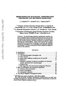
Figure 1: The left plot shows comparison of the constant step-size αP as function of σA found by Algorithm 1 versus the constant step-size computed in closed form. The right plot shows the performance of LSA with CS-PR (with the step-size choosen by Algorithm 1) for various σA values. The errors were insignificant and hence error bars are not shown in the right plot. “roughly” (making allowance for the persistent noise) decreasing and converge to 1 when the stepsize is large enough so that the iterates stay bounded and eventually converge. The idea is that the IsU nstable() routine in Algorithm 1 calculates {ri }i based on its input and returns true when any of these is larger than a preset constant c > 1. By choosing a larger the constant c, the probability of false detection of a run-away event decreases rapidly, while still controlling for the probability of altogether missing a run-away event.   1 −10 , σb = 0 and bt = b, ∀t ≥ 0 We ran numerical experiments on the class with AP = 10 1 (chosen such that θ∗ = (1, 1)⊤ ) and Mt , t ≥ 0 with varying σA ’s. This problem class does not admit an apriori step-size (due to the unknown σA and the dependence of step-size on σA ) that prevents the explosion of MSE. The results (see Figure 1) show that Algorithm 1 does find a problem dependent constant step-size (within a factor of the best possible hand computed step-size) that avoids the MSE blow up. We chose k = 2 and T = 5, the preset constant was chosen to be 1.025 and the results are for σA = 0, 2, 5, 10, 20. Algorithm 1 is oblivious of the data distribution, and the hand computed step-size is based on full problem information (i.e., σA ). Further, the results (in the right plot of Figure 1) also confirm our expectation that higher step-sizes lead to faster convergence.

8 Conclusion We presented a finite time performance analysis of LSAs with CS-PR and showed that the MSE decays at a rate O( 1t ). Our results extended the analysis of Dieuleveut et al. [4] for SGD with CS-PR for the problem of linear least-squares estimation and i.i.d. sampling to general LSAs with CS-PR. Due to the lack of special structures, our analysis for the case of general LSA cannot recover entirely the results of Dieuleveut et al. [4] who use the problem specific structures in their analysis. Our results also improved the rates in the case of the GTD class of algorithms. We presented conditions under which a constant step-size can be chosen uniformly for a given class of data distributions. We showed a negative result in that not all data distributions ‘admit’ such a constant step-size. This is a 8

negative result from the perspective of TD algorithms in RL. We also argued that a problem dependent constant step-size can be obtained in an automatic manner and presented numerical experiments on a synthetic LSA.

References [1] Francis R Bach and Eric Moulines. Non-asymptotic analysis of stochastic approximation algorithms for machine learning. In Advances in Neural Information Processing Systems, pages 451–459, 2011. [2] Christoph Dann, Gerhard Neumann, and Jan Peters. Policy evaluation with temporal differences: a survey and comparison. Journal of Machine Learning Research, 15(1):809–883, 2014. [3] Alexandre Défossez and Francis Bach. Averaged least-mean-squares: Bias-variance trade-offs and optimal sampling distributions. In Artificial Intelligence and Statistics, pages 205–213, 2015. [4] Aymeric Dieuleveut, Nicolas Flammarion, and Francis Bach. Harder, better, faster, stronger convergence rates for least-squares regression. arXiv preprint arXiv:1602.05419, 2016. [5] Simon S Du, Jianshu Chen, Lihong Li, Lin Xiao, and Dengyong Zhou. Stochastic variance reduction methods for policy evaluation. arXiv preprint arXiv:1702.07944, 2017. [6] Vijay R Konda and John N Tsitsiklis. Linear stochastic approximation driven by slowly varying Markov chains. Systems & Control Letters, 50(2):95–102, 2003. [7] Nathaniel Korda and LA Prashanth. On TD(0) with function approximation: Concentration bounds and a centered variant with exponential convergence. In ICML, pages 626–634, 2015. [8] Sascha Lange, Thomas Gabel, and Martin Riedmiller. Batch reinforcement learning. In Reinforcement learning, pages 45–73. Springer, 2012. [9] Yitao Liang, Marlos C. Machado, Erik Talvitie, and Michael H. Bowling. State of the art control of atari games using shallow reinforcement learning. In AAMAS, pages 485–493, 2016. [10] Long-Ji Lin. Self-improving reactive agents based on reinforcement learning, planning and teaching. Machine learning, 8(3-4):293–321, 1992. [11] Bo Liu, Ji Liu, Mohammad Ghavamzadeh, Sridhar Mahadevan, and Marek Petrik. Finitesample analysis of proximal gradient td algorithms. In UAI, pages 504–513, 2015. [12] Boris T Polyak and Anatoli B Juditsky. Acceleration of stochastic approximation by averaging. SIAM Journal on Control and Optimization, 30(4):838–855, 1992. [13] David Ruppert. Efficient estimations from a slowly convergent robbins-monro process. Technical report, Cornell University Operations Research and Industrial Engineering, 1988. [14] Richard S Sutton and Andrew G Barto. Reinforcement learning: An introduction, volume 1. MIT press Cambridge, 1998. [15] Richard S Sutton, Hamid R Maei, and Csaba Szepesvári. A convergent o(n) temporaldifference algorithm for off-policy learning with linear function approximation. In Advances in neural information processing systems, pages 1609–1616, 2009. [16] Richard S Sutton, Hamid Reza Maei, Doina Precup, Shalabh Bhatnagar, David Silver, Csaba Szepesvári, and Eric Wiewiora. Fast gradient-descent methods for temporal-difference learning with linear function approximation. In Proceedings of the 26th Annual International Conference on Machine Learning, pages 993–1000, 2009. [17] John N Tsitsiklis and Benjamin Van Roy. On average versus discounted reward temporaldifference learning. Machine Learning, 49(2):179–191, 2002.

9

A

Linear Algebra Preliminaries

A.1 Additional Notations For x = a + ib ∈ C, we denote its real and imaginary parts by re(x) = a and im(x) = b respectively. Given a x ∈ Cdp , for 1 ≤ i ≤ d, x(i) denotes the ith component of x. For any x ∈ C we denote its modulus |x| = re(x)2 + im(x)2 and its complex conjugate by x ¯ = a−ib. We use A  0 to denote that the square matrix A is Hermitian and positive semidefinite (HPSD): A = A∗ , inf x x∗ Ax ≥ 0. We use A ≻ 0 to denote that the square matrix A is Hermitian and positive definite (HPD): A = A∗ , inf x x∗ Ax > 0. For A, B HPD matrices, A  B holds if A − B  0. We also use A ≻ B similarly to denote that A − B ≻ 0. We also use  and ≺ analogously. We denote the smallest eigen value of a real symmetric positive definite matrix A by λmin (A). We now present some useful results from linear algebra.  B1 0  0 B2 Let B be a d × d block diagonal matrix given by B =  ..  ... . 0 ... Pk di × di matrix such that di < d, ∀i = 1, . . . , k (w.l.o.g) and i=1 di

 0 ... 0 0 ... 0  , where Bi is a ..  .. .. .  . . 0 0 Bk = d. We also denote B as

B = B1 ⊕ B2 ⊕ . . . Bk = ⊕ki=1 Bi

A.2 Results in Matrix Decomposition and Transformation We will now recall Jordon decomposition. Lemma 2. Let A ∈ Cd×d and {λi ∈ C, i = 1, . . . , k ≤ d} denote its k distinct eigenvalues. ˜ −1 , where Λ ˜ = Λ ˜1 ⊕ . . . ⊕ Λ ˜ k, There exists a complex matrix V ∈ Cd×d such that A = V ΛV i i i ˜ ˜ ˜ ˜ ˜ where each Λi , i = 1, . . . , k can further be written as Λi = Λ1 ⊕ . . . ⊕ Λl(i) . Each of Λj , j = P i 1, . . . , l(i) is a dij × dij square matrix such that l(i) j=1 dj = di and has the special form given by   λi 1 0 . . . 0 0 0 λi 1 0 . . . 0   . ˜i =  Λ .. .. j 0 . 0 λ 1 . i

0

... 0

0

0

λi

Lemma 3. Let A ∈ Cd×d be a Hurwitz matrix. There exists a matrix U ∈ GL(d) such that A = U ΛU −1 and Λ∗ + Λ is a real symmetric positive definite matrix.

Proof. It is trivial to see that for any Λ ∈ Cd×d , (Λ∗ + Λ) is Hermitian. We will use the de˜ −1 in Lemma 2 and also carry over the notations in Lemma 2. Concomposition of A = V ΛV   1 0 0 ... 0 0 0 re(λi ) 0 0 ... 0    .. .. sider the diagonal matrices Dji =  i  , ∀j = 1, . . . , l(i), 0 . . 0 re(λ )dj −1 0  i

i

0 ... 0 0 0 re(λi )dj i , ∀i = 1, . . . , k and D = D1 ⊕. . .⊕Dk . It follows that A = (V D)Λ(V D)−1 , Di = D1i ⊕. . .⊕Dl(i) where Λ is a matrix such that Λ = Λ1 ⊕ . . .⊕ Λk , where each Λi , i = 1, . . . , k can further be written as Ai = Λi1 ⊕ . . . ⊕ Λil(i) . Each of Λij is a dij × dij square matrix with the special form given by   λi re(λi ) 0 ... 0 0 λi re(λi ) 0 . . . 0  0 . Λij =  .. .. 0 . . 0 λ re(λ ) i

0

...

0

0

0

i

λi

10

∗

(Λ Now we have  i) re(λi ) re(λ 0 2  re(λi ) re(λi )  2 re(λi ) 2  .. ..   0 . . 0 ... 0 Cd (6= 0), we have ∗ (Λ

x

∗

+Λ) 2

... 0 0 0

= 0 ...

l(i)

⊕ki=1 

⊕j=1

i Λi∗ j +Λj , 2

where

i Λi∗ j +Λj 2

=

0  0  . Then for any x = (x(i), i = 1, . . . , d) ∈  i)  re(λi ) re(λ 2 re(λi ) re(λi ) 2

d−1 d Xx X ¯(i)x(i + 1) + x(i)¯ x(i + 1) + Λ) x¯(i)x(i) + x = re(λi ) 2 2 i=1 i=1

 re(λ ) re(λi )  i 2 2 = |x(1)| + |x(d)| + 2 2 ! d re(λi ) X 2 > |x(i) + x(i + 1)| 2 i=1

d−1 X

!

2

|x(i)| + x ¯(i)x(i + 1) + x(i)¯ x(i + 1) + |x(i + 1)|

i=1

>0

B Proofs B.1

LSA with CS-PR for Positive Definite Distributions

In this subsection, we re-write (2) and Assumption 1 to accomodate complex number computations and in addition assume that P is positive definite. To this end, θt = θt−1 + α(bt − At θt−1 ), 1 Xt θi , θˆt = i=0 t+1

LSA: PR-Average: where θˆt , θt ∈ Cd . We now assume,

(4a) (4b)

Assumption 2. 1. (bt , At ) ∼ (P b , P A ), t ≥ 0 is an i.i.d. sequence, where P b is a distribution over Cd and P A is a distribution over Cd×d . We assume that P is positive definite. ·

·

2. The martingale difference sequences7 Mt = At − AP and Nt = bt − bP associated with At and bt satisfy the following i h 2 2 , E[Nt∗ Nt ] = σb2P . E kMt k | Ft−1 ≤ σA P 3. AP is invertible and there exists a θ∗ = A−1 P bP . We now define the error variables and present the recurison for the error dynamics. In what follows, definitions in Section 2 and Section 3 continue to hold. Definition 7. · · • Define error variables et = θt − θ∗ and eˆt = θˆt − θ∗ . ·

• Define ∀ t ≥ 0 random vectors ζt = bt − b − (At − AP )θ∗ . i h · · 2 2 2 2 kθ∗ k. Note that E kζt k ≤ σ12 and kθ∗ k + σb2 and σ22 = σA • Define constants σ12 = σA E [kMt ζt k] ≤ σ22 .

• Define ∀ i ≥ j, the random matrices Fi,j = (I − αAi ) . . . (I − αAj ) and ∀, i < j Fi,j = I. 7

E [Mt |Ft−1 ] = 0 and E [Nt |Ft−1 ] = 0

11

2

!

Error Recursion Let us now look at the dynamics of the error terms defined by
θt = θt−1 + α bt − At θt−1
θt − θ∗ = θt−1 − θ∗ + α bt − At (θt−1 − θ∗ + θ∗ ) et = (I − αAt )et−1 + α(bt − b − (At − A)θ∗ ) et = (I − αAt )et−1 + αζt

(5)

Lemma 4. Let P be a distribution over Cd × Cd×d satisfying Assumption 2, then there exists an αP > 0 such that ρd (α, P ) > 0 and ρs (α, P ) > 0, ∀α ∈ (0, αP ). Proof. (a)

ρs (α, P ) =

(b)

=

inf

x∗ (A∗P + AP )x − αx∗ E [A∗t At ] x

inf

x∗ (A∗P + AP )x − αx∗ A∗P AP − αx∗ E [Mt∗ Mt ] x

x:kxk=1

x:kxk=1

(c)

2

2 ≥ λmin (A∗P + AP ) − α kAP k − σA λ

(A∗ +A )

P P The proof is complete by choosing αP < min . Here (a) follows from definition of 2 kAP k2 +σA ρs (α, P ) in Definition 1, (b) follows from the fact that Mt is a martingale difference term (see Assumption 2) and (c) follows from the fact that for a real symmetric matrix M the smallest eigen value is given by λmin = inf x:kxk=1 x∗ M x.

Lemma 5 (Product unroll lemma). Let t > i ≥ 1, x, y ∈ Cd be Fi -measurable random vectors. Then, E[x∗ Ft,i+1 y|Fi ] = x∗ (I − αAP )t−i y . Proof. By the definition of Ft,i+1 , and because Ft−1,i+1 = (I − αAt−1 ) . . . (I − αAi+1 ) is Ft−1 measurable, as are x and y, E [x∗ Ft,i+1 y|Ft−1 ] = x⊤ E [(I − αAt )|Ft−1 ] Ft−1,i+1 y = x∗ (I − αAP )Ft−1,i+1 y . By the tower-rule for conditional expectations and our measurability assumptions, E [x∗ Ft,i+1 y|Ft−2 ] = x∗ (I − αAP )E [Ft−1,i+1 |Ft−2 ] y = x∗ (I − αAP )2 Ft−2,i+1 y . Continuing this way we get E [x∗ Ft,i+1 y|Ft−j ] = x∗ (I − αAP )j Ft−j,i+1 y ,

j = 1, 2, . . . , t − i .

Specifically, for j = t − i we get E [x∗ Ft,i+1 y|Fi ] = x∗ (I − αAP )t−i y . Lemma 6. Let t > i ≥ 1 and let x ∈ Cd be a Fi−1 -measurable random vector. Then, E[x∗ Ft,i+1 ζi ] = 0. Proof. By Lemma 5, E [x∗ Ft,i+1 ζi |Fi ] = x∗ (I − αAP )t−i ζi . Using the tower rule, E [x∗ Ft,i+1 ζi |Fi−1 ] = x∗ (I − αAP )t−i E [ζi |Fi−1 ] = 0 . Lemma 7. For all t > i ≥ 0, Ehei , Ft,i+1 ei i = Ehei , (I − αAP )t−i ei i. 12

Proof. The lemma follows directly from Lemma 5. Indeed, θi depends only on A1 , . . . , Ai , b1 , . . . , bi , θi and so is ei Fi -measurable. Hence, the lemma is applicable and implies that   E [hei , Ft,i+1 ei i|Fi ] = E hei , (I − αAP )t−i ei i|Fi .

Taking expectation of both sides gives the desired result.

Lemma 8. Let i > j ≥ 0 and let x ∈ Rd be an Fj -measurable random vector. Then, 2

EhFi,j+1 x, Fi,j+1 xi ≤ (1 − αρs (α, P ))i−j E kxk . . Proof. Note that St = E [(I − αAt )∗ (I − αAt )|Ft−1 ] = I − α(A∗P + AP ) + α2 E [A∗t At |Ft−1 ]. Since (bt , At )t is an independent sequence, E [A∗t At |Ft−1 ] = E [A∗1 A1 ]. Now, using the definition of ρs (α, P ) from Definition 1 supx:kxk=1 x⊤ St x = 1 − α inf x:kxk=1 x⊤ (A∗P + AP −   αE A⊤ 1 A1 )x = 1 − αρs (α, P ). Hence, E [hFi,j+1 x, Fi,j+1 xi|Fi−1 ]   ⊤ = E x∗ Fi−1,j+1 (I − αAi )∗ (I − αAi )Fi−1,j+1 x | Fi−1 = (xFi−1,j+1 )∗ Si Fi−1,j+1 x ≤ (1 − αρs (α, P )) hFi−1,j+1 x, Fi−1,j+1 xi

≤ (1 − αρs (α, P ))2 hFi−2,j+1 x, Fi−2,j+1 xi .. . ≤ (1 − αρs (α, P ))i−j kxk2 .

Theorem 3. Let eˆt be as in Definition 7. Then   1 2 2 E[kˆ et k ] ≤ 1 + αρd (α, P ) αρs (α, P )

2

ke0 k α2 (σ12 ) + ασ22 ke0 k + (t + 1)2 t+1

!

.

(6)

Proof. et = (I − αAt )(I − αAt−1 )et−2 + α(I − αAt )ζt−1 + αζt .. . = (I − αAt ) · · · (I − αA1 )e0 + α(I − αAt ) · · · (I − αA2 )ζ1 + α(I − αAt ) · · · (I − αA3 )ζ2 .. . + αζt , which can be written compactly as et = Ft,1 e0 + α(Ft,2 ζ1 + · · · + Ft,t+1 ζt ) , eˆt =

1 nXt 1 Xt Fi,1 e0 ei = i=0 i=0 t+1 t+1 ! t t o X X Fk,i+1 ζi , +α i=1

13

k=i

(7)

where in the second sum we flipped the order of sums and swapped the names of the variables that the sum runs over. It follows that t X 1 2 E[kˆ et k ] = Ehˆ et , eˆt i = Ehei , ej i . (t + 1)2 i,j=0

Hence, we see that it suffices to bound E [hei , ej i]. There are two cases depending on whether i = j. When i < j,   P Ehei , ej i = Ehei , Fj,i+1 ei + α jk=i+1 Fj,k+1 ζk i = Ehei , Fj,i+1 ei i(from Lemma 6)

= Ehei , (I − αA)j−i ei i(from Lemma 7) and therefore t−1 X t X

Ehei , ej i =

i=0 j=i+1

≤ Since

P

i,j

·=

Xt−1 1 Ehei , ei i i=0 αρd (α, P )

Xt 2 Ehei , ei i . i=0 αρd (α, P )

P P · + 2 i j>i ·,  Xt Xt Ehei , ej i = 1 +

P

i=j

X t 2 Ehei , ei i . j=0 i=0 i=0 αρd (α, P ) Expanding ei using (7) and then using Lemma 8 and Assumption 2 Ehei , ei i = EhFi,1 e0 , Fi,1 e0 i + α2

Xi

2

j=1

≤ (1 − αρs (α, P ))i ke0 k + α2 and so Xt

i=0

Xt

j=0

Ehei , ej i ≤

Putting things together,  2 E[kˆ et k ] ≤ 1 +

 1+

EhFi,j+1 ζj , Fi,j+1 ζj i + α



EhFi,1 e0 , Fi,j+1 ζj i

j=1

σ12 σ 2 ke0 k +α 2 , αρs (α, P ) αρs (α, P )

2 αρd (α, P )

2 αρd (α, P )

i X



1 (t(α2 σ12 + ασ22 ke0 k) + ke0 k2 ) . αρs (α, P )

1 αρs (α, P )

2

ke0 k α2 (σ12 ) + ασ22 ke0 k + (t + 1)2 t+1

!

.

(8)

Proof of Lemma 1 Lemma 9. Let P be a distribution over Rd × Rd×d satisfying Assumption 1, then there exists an αPU > 0 and U ∈ GL(d) such that ρd (α, PU ) > 0 and ρs (α, PU ) > 0, ∀α ∈ (0, αP ). Proof. We know that AP is Hurwitz and from Lemma 3 it follows that there exists an U ∈ GL(d) such that Λ = U −1 AP U and (Λ∗ + Λ) is real symmetric and positive definite. Using Definition 2, we have APU = Λ and from Lemma 4 we know that there exists an αPU such that ρd (α, PU ) > 0 and ρs (α, PU ) > 0, ∀α ∈ (0, αPU ). Lemma 10 (Change of Basis). Let P be a distribution over Rd × Rd×d as in Assumption 1 and let · · U be chosen according to Lemma 1. Define γt = U −1 θt , , γ∗ = U −1 θ∗ , then !

 2 2 i  h

U −1 2 kθ0 − θ∗ k α2 (σP2 kθ∗ k + σb2 ) + α(σP2 kθ∗ k) kθ0 − θ∗ k 2 2 . + E kγt − γ∗ k ≤ 1 + αρd (α, PU ) αρs (α, PU ) (t + 1)2 t+1 (9) P t 1 where γˆt = t+1 s=0 γs . 14

·

Proof. Consider the modified error recursion in terms of zt = γt − γ∗ et = (I − αAt )et−1 + αζt U −1 et = (I − αU −1 At U )U −1 et−1 + αU −1 ζt zt = (I − αΛt )zt−1 + αHt ,

(10)

where Λt = U −1 At U and Ht = U −1 ζt . Note that the error recursion in zt might involve complex computations (depending on whether U has complexhentriesior not), and hence (4) and

2 2 ≤ U −1 E [kζt k] and Assumption 2 are useful in analyzing zt . We know that E kHt k





   E [kΛt Ht k] = E U −1 At U U −1 ζt = E U −1 At ζt ≤ U −1 E [kAt ζt k] = U −1 σ22 . Pt · 1 Now applying Theorem 3 to zˆt = t+1 s=0 zt , we have !

2

  2 α2 ( U −1 σ12 ) + α( U −1 σ22 ) kz0 k 2 kz0 k 1 2 E[kˆ zt k ] ≤ 1 + + αρd (α, PU ) αρs (α, PU ) (t + 1)2 t+1 (11) !

−1 2



  2 2

U ke0 k α2 ( U −1 σ12 ) + α( U −1 σ22 ) U −1 ke0 k 1 2 + ≤ 1+ αρd (α, PU ) αρs (α, PU ) (t + 1)2 t+1 (12)

Follows by substituting θt = U γt in Lemma 10.

Proof of Theorem 1

Proof of Theorem 2 Consider the LSA with (bt , At ) ∼ P such that bt = (Nt , 0)⊤ ∈ R2 is a zero mean i.i.d. random variable with variance σb2 , and At = A, ∀t ≥ 0, where A = AP =   λmin 0 , for some λmax > λmin > 0. Note that in this example θ∗ = 0. By choosing 0 λmax 2 , in this case it is straightforward to write the expression for eˆt explicitly as below: α < λmax t t t X t X 1 X 1 X (I − αAP )i−s bs et = (I − αAP )t−s e0 + t + 1 s=0 t + 1 s=0 s=1 i=s # " t X

1 t+1−s t+1 −1 = bs . I − (I − αAP ) e0 + I − (I − αAP ) (αAP ) t+1 s=1

eˆt =

Thus,

h
1

(αAP )−1 I − (I − αAP )t+1 e0 2 2 (t + 1) t X


i

(αAP )−1 I − (I − αAP )t+1−s bs 2 , +

i (a) h E kˆ et k2 =

s=1

and hence

h
2 1 −2 1 − (1 − αλmin )t+1 θ02 (1) (αλ ) min (t + 1)2 t i X
2 1 − (1 − αλmin )t+1−s b2s (1) .

i h   (b) 2 E kˆ et k ≥ E eˆ2t (1) = +

1 (t + 1)2

s=1

Here (a) and (b) follows from the i.i.d. assumption. Note that in this example, ρs (α, P ) = 2 ρd (α, P ) = 2λmin − αλ2min = λmin (2 − αλmin ), and kθ∗ k = 0 and σA = 0. Further, the re2 2 sult follows by noting the fact that noting the fact that kbt k = bt (1) and kθt k2 = θt (1)2 . Proof of Proposition 1 Fix an arbitrary α > 0. We show that there exists P ∈ P such that ρα (P ) < 0. For ǫ ∈ (0, 1/2) let P = (P V , P M ) be the distribution such that P M is supported on {−I, I} and takes on the value of I with probability 1/2 + ǫ. Then AP = 2ǫI ≻ 0, hence P ∈ P1 . Further, QP = I. Hence, ρs (α, P ) = 4ǫ − α. Hence, if ǫ < α/4, ρα (P ) < 0. 15

Proof of Proposition 2 Since PPSD,B is supported on the set of positive semi-definite matrices, we know for any A ∈ Rd×d that is PSD, we can consider the SVD of A: A = U ΛU ⊤ where U is orthonormal and Λ is diagonal with nonnegative elements. Note that Λ  B I and thus Λ2  BΛ. Then for any x ∈ Rd , x⊤ A⊤ Ax = x⊤ U Λ2 U ⊤ x ≤ Bx⊤ U ΛU ⊤ x = Bx⊤ Ax. Taking expectations we find that x⊤ CP x ≤ Bx⊤ AP x. Hence, ρs (α, PPSD,B ) = 2x⊤ AP x − αx⊤ CP x ≥ (2 − αB) x⊤ AP x. Thus, for any α < 2/B, ρα (P ) > 0. Proof of Proposition 3

Consider the case when the smallest eigenvalue of AP is 0.

16