Linking Pose and Motion*. Andrea Fossati and Pascal Fua. Computer Vision Laboratory. Ãcole Polytechnique Fédérale de Lausanne (EPFL). 1015 Lausanne ...
Linking Pose and Motion? Andrea Fossati and Pascal Fua Computer Vision Laboratory ´ Ecole Polytechnique F´ed´erale de Lausanne (EPFL) 1015 Lausanne, Switzerland {andrea.fossati, pascal.fua}@epfl.ch
Abstract. Algorithms designed to estimate 3D pose in video sequences enforce temporal consistency but typically overlook an important source of information: The 3D pose of an object, be it rigid or articulated, has a direct influence on its direction of travel. In this paper, we use the cases of an airplane performing aerobatic maneuvers and of pedestrians walking and turning to demonstrate that this information can and should be used to increase the accuracy and reliability of pose estimation algorithms.
1
Introduction
Temporal consistency is a key ingredient in many 3D pose estimation algorithms that work on video sequences. However, the vast majority of methods we know of neglect an important source of information: The direction in which most objects travel is directly related to their attitude. This is just as true of the fighter plane of Fig. 1(a) that tends to move in the direction in which its nose points as of the pedestrian of Fig. 1(b) who is most likely to walk in the direction he is facing. The relationship, though not absolute—the plane can slip and the pedestrian can move sideways—provides nevertheless useful constraints. There are very many Computer Vision papers on rigid, deformable, and articulated motion tracking, as recent surveys can attest [1, 2]. In most of these, temporal consistency is enforced by regularizing the motion parameters, by relating parameters in an individual frame to those estimated in earlier ones, or by imposing a global motion model. However, we are not aware of any that explicitly take the kind of constraints we propose into account without implicitly learning it from training data, as is done in [3]. In this paper, we use the examples of the plane and the pedestrian to show that such constraints, while simple to enforce, effectively increase pose estimation reliability and accuracy for both rigid and articulated motion. In both cases, we use challenging and long video sequences that are shot by a single moving camera ?
This work has been funded in part by the Swiss National Science Foundation and in part by the VISIONTRAIN RTN-CT-2004-005439 Marie Curie Action within the EC’s Sixth Framework Programme. The text reflects only the authors’ views and the Community is not liable for any use that may be made of the information contained therein.
2
Andrea Fossati and Pascal Fua
(a)
(b)
Fig. 1. Airplanes and people are examples of objects that exhibit a favored direction of motion. (a) We project the 3D aircraft model using the recovered pose to produce the white overlay. The original images are shown in the upper right corner. (b) We overlay the 3D skeleton in the recovered pose, which is correct even when the person is occluded.
that can zoom to keep the target object in the field of view, rendering the use of simple techniques such as background subtraction impractical.
2
Related Work and Approach
Non-holonomic constraints that link direction of travel and position have been widely used in fields such as radar-based tracking [4] or robot self-localization [5], often in conjunction with Kalman filtering. However, these approaches deal with points moving in space and do not concern themselves with the fact that they are extended 3D objects, whether rigid or deformable, that have an orientation, which conditions the direction in which they move. Such constraints have also been adopted for motion synthesis in the Computer Graphics community [6], but they are not directly applicable in a Computer Vision context since they make no attempt at fitting model to data.
Linking Pose and Motion
3
Tracking rigid objects in 3D is now a well understood problem and can rely on many sources of image information, such as keypoints, texture, or edges [1]. If the image quality is high enough, simple dynamic models that penalize excessive speed or acceleration or more sophisticated Kalman filtering techniques [7] are sufficient to enforce temporal consistency. However, with lower quality data such as the plane videos of Fig. 1(a), the simple quadratic regularization constraints [8] that are used most often yield unrealistic results, as shown in Fig. 2.
(a)
(b)
(c)
Fig. 2. The first 50 frames of the first airplane sequence. The 3D airplane model is magnified and plotted once every 5 frames in the orientation recovered by the algorithm: (a) Frame by Frame tracking without regularization. (b) Imposing standard quadratic regularization constraints. (c) Linking pose to motion produces a much more plausible set of poses. Note for example the recovered depth of the brightest airplane: In (a) and (b) it appears to be the frontmost one, which is incorrect. In (c) the relative depth is correctly retrieved.
Tracking a complex articulated 3D object such as a human body is much more complex and existing approaches remain brittle. Some of the problems are caused by joint reflection ambiguities, occlusion, cluttered backgrounds, non-rigidity of tissue and clothing, complex and rapid motions, and poor image resolution. The problem is particularly acute when using a single video to recover the 3D motion. In this case, incorporating motion models into the algorithms has been shown to be effective [2]. The models can be physics-based [9] or learned from training data [10–13]. However, all of these assume the joint angles, that define the body pose, and the global motion variables are independent. As is the case for rigid body tracking, they typically revert to second order Gauss-Markov modeling or Kalman filtering to smooth the global motion. Again, this can lead to unrealistic results as shown in Fig. 3. Some approaches implicitly take into account the relationship between pose and direction of travel by learning from training data a low-dimensional representation that includes both [3, 14–16]. However, the set of motions that can be represented is heavily constrained by the contents of the training database, which limits their generality.
4
Andrea Fossati and Pascal Fua
(a)
(b)
Fig. 3. Recovered 2D trajectory of the subject of Fig. 1(b). The arrows represent the direction he is facing. (a) When pose and motion are not linked, he appears to walk sideways. (b) When they are, he walks naturally. The underlying grid is made of 1 meter squares.
To remedy these problems, we explicitly link pose and motion as follows: Given an object moving along its trajectory as depicted by Fig. 4, the angle between P˙t, the derivative of its position, and its orientation Λt should in general be small. We can therefore write that P˙t · Λt ||P˙ t|| · ||Λt|| should be close to 1. To enforce this, we can approximate the derivative of the locations using finite differences between estimated locations Pˆ at different time instants. This approximation is appropriate when we can estimate the location at a sufficiently high frequency (e.g. 25 Hz). Our constraint then reduces to minimizing the angle between the finite differences approximation of the derivative of the trajectory at time t, given by Pˆt+1 − Pˆt , and the object’s estimated orientation given by Λˆt. We write this angle, which is depicted as filled both at time t − 1 and t in Fig. 4, as
φt→t+1 = acos
Pˆ˙t · Λˆt (Pˆt+1 − Pˆt ) · Λˆt = acos ||(Pˆt+1 − Pˆt )|| · ||Λˆt|| ||Pˆ˙t|| · ||Λˆt||
and will seek to minimize it. It is important to note that the constraint we impose is not a hard constraint, which can never be violated. Instead, it is a prior that can be deviated from if the data warrants it. In the remainder of the paper we will demonstrate the effectiveness of this idea for both rigid and articulated 3D tracking.
Linking Pose and Motion
5
Fig. 4. The continuous curve represents the real trajectory of the object, while the dashed lines show its approximation by finite differences.
3
Rigid Motion
In the case of a rigid motion, we demonstrate our approach using video sequences of a fighter plane performing aerobatic maneuvers such as the one depicted by Fig. 5. In each frame of the sequences, we retrieve the pose which includes position expressed by cartesian coordinates and orientation defined by the roll, pitch and yaw angles. We show that these angles can be recovered from single viewpoint sequences with a precision down to a few degrees, and that linking pose and motion estimation contributes substantially to achieving this level of accuracy. This is extremely encouraging considering the fact that the videos we have been working with were acquired under rather unfavorable conditions: As can be seen in Fig. 5, the weather was poor, the sky gray, and the clouds many, all of which make the plane less visible and therefore harder to track. The airplane is largely occluded by smoke and clouds in some frames, which obviously has an adverse impact on accuracy but does not result in tracking failure. The video sequences were acquired using a fully calibrated camera that could rotate around two axes and zoom on the airplane. Using a couple of encoders, it could keep track of the corresponding values of the pan and tilt angles, as well as the focal length. We can therefore consider that the intrinsic and extrinsic camera parameters are known in each frame. In the remainder of this section, we present our approach first to computing poses in individual frames and then imposing temporal consistency, as depicted by Fig. 4, to substantially improve the accuracy and the realism of the results. 3.1
Pose in Each Frame Independently
Since we have access to a 3D model of the airplane, our algorithm computes the pose in each individual frame by minimizing an objective function Lr that is a weighted sum of a color and an edge term:
6
Andrea Fossati and Pascal Fua
Fig. 5. Airplane video and reprojected model. First and third rows: Frames from the input video. Note that the plane is partially hidden by clouds in some frames, which makes the task more difficult. Second and fourth rows: The 3D model of the plane is reprojected into the images using the recovered pose parameters. The corresponding videos are submitted as supplemental material.
– The color term is first computed as the Bhattacharyya distance [17] between the color histogram of the airplane that we use as a model, whose pose was captured manually in the first frame, and the color histogram of the image area corresponding to its projection in subsequent frames. To this we add a term that takes into account background information, also expressed as a difference of color histograms, which has proved important to guarantee robustness. – The edge term is designed to favor poses such that projected model edges correspond to actual image edges and plays an important role in ensuring accuracy. In each frame t, the objective function Lr is optimized using a particle-based stochastic optimization algorithm [18] that returns the pose corresponding to the best sample. The resulting estimated pose is a six-dimensional vector Sˆt =
Linking Pose and Motion
7
ˆt , Yˆt , Zˆt) is the estimated position of (Pˆt, Λˆt) = argminS Lr (S) where Pˆt = (X the plane in an absolute world coordinate system and Λˆt = (ˆ ρt , θˆt , γˆt) is the estimated orientation expressed in terms of roll, pitch and yaw angles. The estimated pose Sˆt at time t is used to initialize the algorithm in the following frame t + 1, thus assuming that the motion of the airplane between two consecutive frames is relatively small, which is true in practice. 3.2
Imposing Temporal Consistency
Independently optimizing Lr in each frame yields poses that are only roughly correct. As a result, the reconstructed motion is extremely jerky. To enforce temporal consistency, we introduce a regularization term M defined over frames t − 1, t, and t + 1 as M (St ) = α1 ||A(Pt)||2 + α2 ||A(Λt)||2 + β(φ2t−1→t + φ2t→t+1 ) ,
(1)
A(Pt ) = Pt+1 − 2Pt + Pt−1 ,
(2)
A(Λt ) = Λt+1 − 2Λt + Λt−1 .
(3)
The first two terms of (1) enforce motion smoothness. The third term is the one of Fig. 4, which links pose to motion by forcing the orientation of the airplane to be consistent with its direction of travel. In practice, α1 , α2 and β are chosen to relate quantities that would otherwise be incommensurate and are kept constant for all the sequences we used. For an N -frame video sequence, ideally, we should minimize fr (S1 , . . . , SN ) =
N X t=1
Lr (St ) +
N −1 X
M (St )
(4)
t=2
with respect to the poses in individual images. In practice, for long video sequences, this represents a very large optimization problem. Therefore, in our current implementation, we perform this minimization in sliding temporal 3frame windows using a standard simplex algorithm that does not require the computation of derivatives. We start with the first set of 3 frames, retain the resulting pose in the first frame, slide the window by one frame, and iterate the process using the previously refined poses to initialize each optimization step. 3.3
Tracking Results
The first sequence we use for the evaluation of our approach is shown in Fig. 5 and contains 1000 frames shot over 40 seconds, a time during which the plane performs rolls, spins and loops and undergoes large accelerations. In Fig. 6(a) we plot the locations obtained in each frame independently. In Fig. 6(b) we imposed motion smoothness by using only the first two terms of (1). In Fig 6(c) we link pose to motion by using all three terms of (1). The trajectories are roughly similar in all cases. However, using the full set of constraints yields a trajectory that is both smoother and more plausible.
8
Andrea Fossati and Pascal Fua
(a)
(b)
(c)
Fig. 6. Recovered 3D trajectory of the airplane for the 40s sequence of Fig. 5: (a) Frame by Frame tracking. (b) Imposing motion smoothness. (c) Linking pose to motion. The coordinates are expressed in meters.
In Fig. 2, we zoom in on a portion of these 3 trajectories and project the 3D plane model in the orientation recovered every fifth frame. Note how much more consistent the poses are when we use our full regularization term. The plane was equipped with sophisticated gyroscopes which gave us meaningful estimates of roll, pitch, and yaw angles, synchronized with the camera and available every third frame. We therefore use them as ground truth. Table 1 summarizes the deviations between those angles and the ones our algorithm produces for the whole sequence. Our approach yields an accuracy improvement over frame by frame tracking as well as tracking with simple smoothness constraint. The latter improvement is in the order of 5 %, which is significant if one considers that the telemetry data itself is somewhat noisy and that we are therefore getting down to the same level of precision. Most importantly, the resulting sequence does not suffer from jitter, which plagues the other two approaches, as can be clearly seen in the videos given as supplemental material. Table 1. Comparing the recovered pose angles against gyroscopic data for the sequence of Fig. 5. Mean and standard deviation of the absolute error in the 3 angles, in degrees. Roll Angle Error Mean Std. Dev. Frame by Frame 2.291 2.040 Smoothness Constraint only 2.092 1.957 Linking Pose to Motion 1.974 1.878
Pitch Angle Error Mean Std. Dev. 1.315 1.198 1.031 1.061 0.975 1.000
Yaw Angle Error Mean Std. Dev. 3.291 2.245 3.104 2.181 3.003 2.046
In Fig. 7 we show the retrieved trajectory for a second sequence, which lasts 20 seconds. As before, in Table 2, we compare the angles we recover against gyroscopic data. Again, linking pose to motion yields a substantial improvement.
Linking Pose and Motion
(a)
(b)
9
(c)
Fig. 7. Recovered 3D trajectory of the airplane for a 20s second sequence: (a) Frame by Frame tracking. (b) Imposing motion smoothness. (c) Linking pose to motion. The coordinates are expressed in meters. Table 2. Second sequence: Mean and standard deviation of the absolute error in the 3 angles, in degrees. Roll Angle Error Mean Std. Dev. Frame by Frame 3.450 2.511 Smoothness Constraint only 3.188 2.445 Linking Pose to Motion 3.013 2.422
4
Pitch Angle Error Mean Std. Dev. 1.607 1.188 1.459 1.052 1.390 0.822
Yaw Angle Error Mean Std. Dev. 3.760 2.494 3.662 2.237 3.410 2.094
Articulated Motion
To demonstrate the effectiveness of the constraint we propose in the case of articulated motion, we start from the body tracking framework proposed in [19]. In this work, it was shown that human motion could be reconstructed in 3D by detecting canonical poses, using a motion model to infer the intermediate poses, and then refining the latter by maximizing an image-based likelihood in each frame independently. In this section, we show that, as was the case for rigid motion recovery, relating the pose to the direction of motion leads to more accurate and smoother 3D reconstructions. In the remainder of the section, we first introduce a slightly improved version of the original approach on which our work is based. We then demonstrate the improvement that the temporal consistency constraint we advocate brings about. 4.1
Refining the Pose in Each Frame Independently
We rely on a coarse body model in which individual limbs are modeled as cylinders. Let St = (Pt , Θt) be the state vector that defines its pose at time t, where Θt is a set of joint angles and Pt a 3D vector that defines the position and orien-
10
Andrea Fossati and Pascal Fua
tation of the root of the body in a 2D reference system attached to the ground plane. In the original approach [19], a specific color was associated to each limb by averaging pixel intensities in the projected area of the limb in the frames where a canonical pose was detected. Then St was recovered as follows: A rough initial state was predicted by the motion model. Then the sum-of-squared-differences between the synthetic image, obtained by reprojecting the model, and the actual one was minimized using a simple stochastic optimization algorithm. Here, we replace the single color value associated to each limb by a histogram, hereby increasing generality. As in Sect. 3.1, we define an objective function La that measures the quality of the pose using the Bhattacharyya distance to express the similarity between the histogram associated to a limb and that of the image portion that corresponds to its reprojection. Optimizing La in each frame independently leads, as could be expected, to a jittery reconstruction as can be seen in the video given as supplemental material. 4.2
Imposing Temporal Consistency
In order to improve the quality of our reconstruction, we perform a global optimization on all N frames between two key-pose detections, instead of minimizing La independently in each frame. To model the relationship between poses we learn a PCA model from a walking database and consider a full walking cycle as a single data point in a low-dimensional space [20, 11]. This lets us parameterize all the poses Si between consecutive key-pose detections by n PCA coefficients (α1 . . . αn), plus a term, η, that represents possible variations of the walking speed during the walking cycle (n = 5 in our experiments). These coefficients do not take into account the global position and orientation of the body, which needs to be parameterized separately. Since the walking trajectory can be obtained by a 2D spline curve lying on the ground plane, defined by the position and orientation of the root at the two endpoints of the sequence, modifying these endpoints Pstart and Pend will yield different trajectories. The root position and orientation corresponding to the different frames will then be picked along the spline curve according to the value of η. It in fact defines where in the walking cycle the subject is at halftime between the two detections. For a constant speed during a walking cycle the value of η is 0.5, but it can go from 0.3 to 0.7 depending on change in speed between the first and the second half-cycle. We can now formulate an objective function that includes both the image likelihood and a motion term, which, in this case, constrains the person to move in the direction he is facing. This objective function is then minimized with respect to the parameters introduced above (α1, . . . , αn, Pstart, Pend, η) on the full sequence between two consecutive key-pose detections. In other words, we seek to minimize
fa (S1 , . . . , SN ) =
N X t=1
La (St ) +
N X t=2
β(φ2t−1→t)
(5)
Linking Pose and Motion
11
with respect to (α1, . . . , αn, Pstart, Pend, η), where the second term is defined the same way as in the airplane case and β is as before a constant weight that relates incommensurate quantities. The only difference is that in this case both the estimated orientation and the expected motion, that define the angle φ, are 2-dimensional vectors lying on the ground plane. This term is the one that links pose to motion. Note that we do not need quadratic regularization terms such as the first two of (1) because our parameters control the entire trajectory, which is guaranteed to be smooth.
4.3
Tracking Results
We demonstrate our approach on a couple of very challenging sequences. In the sequence of Fig. 8, the subject walks along a circular trajectory and the camera is following him from its center. At a certain point the subject undergoes a total occlusion but the algorithm nevertheless recovers his pose and position thanks to its global motion model. Since the tracking is fully 3D, we can also recover the trajectory of the subject on the ground plane and his instantaneous speed at each frame. In Fig. 3 we examine the effect of linking or not pose to motion on the recovered trajectory: That is, setting β to zero or not in (5). The arrows represent the orientation of the subject on the ground plane. They are drawn every fifth frame. The images clearly show that, without temporal consistency constraints, the subject appears to slide sideways while when the constraints are enforced the motion is perfectly consistent with the pose. This can best be evaluated from the videos given as supplemental material. To validate our results, we manually marked the subject’s feet every 10 frames in the sequence of Fig. 8 and used their position with respect to the tiles on the ground plane to estimate their 3D coordinates. We then treated the vector joining the feet as an estimate of the body orientation and the midpoint as an estimated of its location. As can be seen in Table 3, linking pose to motion produces a small improvement in the position estimate and a much more substantial one in the orientation estimate, which is consistent with what can be observed in Fig. 3.
Table 3. Comparing the recovered pose angles against manually recovered ground truth data for the sequence of Fig. 8. It provides the mean and standard deviation of the absolute error in the X and Y coordinates, in centimeters, and the mean and standard deviation of the recovered orientation, in degrees. X Error Y Error Orientation Error Mean Std. Dev. Mean Std. Dev. Mean Std. Dev. Not Linking Pose to Motion 12.0 7.1 16.8 11.9 11.7 7.6 Linking Pose to Motion 11.8 7.3 14.9 9.3 6.2 4.9
12
Andrea Fossati and Pascal Fua
Fig. 8. Pedestrian tracking and reprojected 3D model for the sequence of Fig. 1 First and third rows: Frames from the input video. The recovered body pose has been reprojected on the input image. Second and fourth rows: The 3D skeleton of the person is seen from a different viewpoint, to highlight the 3D nature of the results. The numbers in the bottom right corner are the instantaneous speeds derived from the recovered motion parameters. The corresponding videos are submitted as supplementary material.
In the sequence of Fig. 9 the subject is walking along a curvilinear path and the camera follows him, so that the viewpoint undergoes large variations. We are nevertheless able to recover pose and motion in a consistent way, as shown in Fig. 10 which represents the corresponding recovered trajectory.
5
Conclusion
In this paper, we have used two very different applications to demonstrate that jointly optimizing pose and direction of travel substantially improves the quality of the 3D reconstructions that can be obtained from video sequences. We have also shown that we can obtain accurate and realistic results using a single moving camera. This can be done very simply by imposing an explicit constraint that forces the angular pose of the object or person being tracked to be consistent with their
Linking Pose and Motion
13
Fig. 9. Pedestrian tracking and reprojected 3D model in a second sequence. First and third rows: Frames from the input video. The recovered body pose has been reprojected on the input image. Second and fourth rows: The 3D skeleton of the person is seen from a different viewpoint, to highlight the 3D nature of the results. The numbers in the bottom right corner are the instantaneous speeds derived from the recovered motion parameters.
(a)
(b)
Fig. 10. Recovered 2D trajectory of the subject of Fig. 9. As in Fig. 3, when orientation and motion are not linked, he appears to walk sideway (a) but not when they are (b).
14
Andrea Fossati and Pascal Fua
direction of travel. This could be naturally extended to more complex interactions between pose and motion. For example, when a person changes orientation, the motion of his limbs is not independent of the turn radius. Similarly, the direction of travel of a ball will be affected by its spin. Explicitly modeling these subtle but important dependencies will therefore be a topic for future research.
References 1. Lepetit, V., Fua, P.: Monocular model-based 3d tracking of rigid objects: A survey. Foundations and Trends in Computer Graphics and Vision (2005) 2. Moeslund, T.B., Hilton, A., Kr¨ uger, V.: A survey of advances in vision-based human motion capture and analysis. CVIU 104(2) (2006) 90–126 3. Sidenbladh, H., Black, M.J., Sigal, L.: Implicit Probabilistic Models of Human Motion for Synthesis and Tracking. In: ECCV. (2002) 4. Bar-Shalom, Y., Kirubarajan, T., Li, X.R.: Estimation with Applications to Tracking and Navigation. John Wiley & Sons, Inc. (2002) 5. Zexiang, L., Canny, J.: Nonholonomic Motion Planning. Springer (1993) 6. Ren, L., Patrick, A., Efros, A.A., Hodgins, J.K., Rehg, J.M.: A data-driven approach to quantifying natural human motion. ACM Trans. Graph. 24(3) (2005) 7. Koller, D., Daniilidis, K., Nagel, H.H.: Model-Based Object Tracking in Monocular Image Sequences of Road Traffic Scenes. IJCV 10(3) (1993) 257–281 8. Poggio, T., Torre, V., Koch, C.: Computational Vision and Regularization Theory. In: Nature. Volume 317. (1985) 9. Brubaker, M., Fleet, D., Hertzmann, A.: Physics-based person tracking using simplified lower-body dynamics. In: CVPR. (2007) 10. Urtasun, R., Fleet, D., Fua, P.: 3D People Tracking with Gaussian Process Dynamical Models. In: CVPR. (2006) 11. Ormoneit, D., Sidenbladh, H., Black, M., Hastie, T.: Learning and tracking cyclic human motion. In: NIPS. (2001) 12. Agarwal, A., Triggs, B.: Tracking articulated motion with piecewise learned dynamical models. In: ECCV. (2004) 13. Taycher, L., Shakhnarovich, G., Demirdjian, D., Darrell, T.: Conditional Random People: Tracking Humans with CRFs and Grid Filters. In: CVPR. (2006) 14. Rosenhahn, B., Brox, T., Seidel, H.: Scaled motion dynamics for markerless motion capture. In: CVPR. (2007) 15. Brox, T., Rosenhahn, B., Cremers, D., Seidel, H.: Nonparametric density estimation with adaptive, anisotropic kernels for human motion tracking. In: Workshop on HUMAN MOTION Understanding, Modeling, Capture and Animation. (2007) 16. Howe, N.R., Leventon, M.E., Freeman, W.T.: Bayesian reconstructions of 3D human motion from single-camera video. In: NIPS. (1999) 17. Djouadi, A., Snorrason, O., Garber, F.: The quality of training sample estimates of the bhattacharyya coefficient. PAMI 12(1) (1990) 92–97 18. Isard, M., Blake, A.: CONDENSATION - conditional density propagation for visual tracking. IJCV 29(1) (1998) 5–28 19. Fossati, A., Dimitrijevic, M., Lepetit, V., Fua, P.: Bridging the Gap between Detection and Tracking for 3D Monocular Video-Based Motion Capture. In: CVPR. (2007) 20. Urtasun, R., Fleet, D., Fua, P.: Temporal Motion Models for Monocular and Multiview 3–D Human Body Tracking. CVIU 104(2-3) (2006) 157–177