LMgr: A Low-Memory Global Router with Dynamic Topology Update and Bending-Aware Optimum Path Search Jingwei Lu
Chiu-Wing Sham
Department of Computer Science and Engineering University of California, San Diego
[email protected]
Department of Electronic and Information Engineering The Hong Kong Polytechnic University
[email protected]
in terms of a bending-aware routing cost function, which is used in many modern global routers [4], [16], [19]. In this paper, we analyze the above two problems and propose our solutions. Our major contributions are listed as follows.
Abstract—Global routing remains a fundamental physical design problem. We observe that large circuits cause high memory cost1 , and modern routers could not optimize the routing path of each two-pin subnet. In this paper, (1) we develop a dynamic topology update technique to improve routing quality (2) we improve the memory efficiency with negligible performance overhead (3) we prove the non-optimality of traditional maze routing algorithm (4) we develop a novel routing algorithm and prove that it is optimum (5) we design a new global router, LMgr, which integrates all the above techniques. The experimental results on the ISPD 2008 benchmark suite show that LMgr could outperform NTHU2.0, NTUgr, FastRoute3.0 and FGR1.1 on solution quality in 13 out of 16 benchmarks and peak memory cost in 15 out of 16 benchmarks, the average memory reduction over all the benchmarks is up to 77%.
•
•
•
I. I NTRODUCTION Modern global routers are mostly based on the structure of integer linear programming (ILP) or iterative rip-up and re-routing (IRR). Albrecht proposes an ILP-based solution in [3] for the linear programming relaxation of the routing problem. BoxRouter2.0 [6] and CGRIP [17] also integrates ILP solvers to optimize their routing solutions. The IRR structure is more popular and widely used among lots of routers. It applies relaxed constraints at early phases and gradually enhances the routing aggressiveness. NTHU2.0 [4] proposes a region-constrained overflow reduction approach. FastRoute3.0 [19] is highly efficiency-oriented and targets fast routability estimation for placers. MaizeRoute [13] designs and implements an extreme edge-shifting technique for congestion removal. MGR [18] generates routing solutions based on a multi-level grid expansion framework. BFGR [10] dynamically adjusts the Lagrange multipliers for a balance between runtime and quality. Other outstanding academic global routers include NTUgr [5] and FGR [16], etc.. Most of these routers are based on a rectilinear Steiner minimum tree (RSMT) topology, they integrate FLUTE [7] library into their routing engines for a fast RSMT topology generation. Among all the above IRR-based routing techniques, two critical problems are usually ignored (1) memory overhead is not negligible at billion-scale design complexity. Modern routers usually record the net usage of each global edge (gedge) in memory, in order to avoid routing-path overlap. When a gedge track is used or released during rip-up and re-routing, its net-usage record is updated accordingly. Such memory overhead could degrade routing efficiency due to conflict cache miss, memory thrashing or page faults. Moreover, gedge net-usage checking could also consume lots of time. (2) Maze routing is widely used in modern routers to generate the optimum routing path for each two-pin subnet. Dijkstra’s algorithm [9] generates the shortest path for a general graph, which is later modified by Lee [12] for grid maze routing problem. Most modern global routers employ Lee’s algorithm to output the minimum-cost routing path for each two-pin subnet. However, we find that this algorithm is not optimum 1 NTHU2.0
•
•
We develop a dynamic RSMT topology update technique, which enhances routing flexibility and improves routing congestion and wirelength. We develop a new technique to utilize routing information in a more efficient manner. Net usage record stored on gedges will be removed, which reduces memory cost. We prove the non-optimality of Lee’s algorithm in terms of the normal routing cost function, which is widely used in many global routers. We develop a bending-aware optimum path search algorithm for maze routing and prove its optimality. We integrate all the above techniques into a new global router, LMgr, which is based on the IRR structure. We validate our innovations through experiments to measure the routing quality and memory cost. The results show that our approach is good both in theory and practice.
The rest of the paper is organized as follows. Section II introduces the problem formulation of global routing and provides with highlevel analysis. Section III discusses our approach for the dynamic RSMT topology update and the reduction of memory cost. In Section IV, we prove the non-optimality of the traditional maze routing algorithm, and propose a novel algorithm with proof on its optimality. In Section V, we present an overview of LMgr. The experimental results are shown and discussed in Section VI. We reach our conclusion in Section VII.
Fig. 1. (a) The chip is decomposed into rectangular regions, each rectangle represents a gcell. (b) The decomposed chip is formulated as a grid graph, each vertex represents a gcell, each edge represents a gedge consists of routing tracks between adjacent gcells.
[4] consumes 11.7GB peak memory at routing newblue3 [15].
1
TABLE I N OTATIONS . Notations vi si,j gsrc / gsnk esrc / esnk gi ei,j cong ci,j clen i,j hi,j ci,j cbnd Ci Ci,j ri
net n is being re-routed on a gedge e. To avoid routing overlap, the router will check whether n is using e on other subnets of it. ′ ′ • e is used by another subnet s of n. s could share e with s with no additional cost. • e is not used by any other subnet of n. To route s on e will add the cost of e to the total routing cost of s. Routers could avoid routing overlaps by applying the above method. However, to search n in the userlist of e (overlap checking) induces time and memory cost, which challenges system memory capacity (large routing grid) and degrades routing efficiency (searching n on e).
Descriptions The ith vertex of a net. The two-pin subnet connecting vi and vj . The source / sink gcell of a routing path. The source / sink gedge of a routing path. The ith gcell in the grid. The gedge connecting gi and gj . The congestion cost of the gedge ei,j . The wirelength cost of the gedge ei,j . The history factor of cost function ci,j . The total cost of ei,j . The cost of a unit bending. The minimum cost from gsrc to gi . The minimum cost from esrc to ei,j . The optimum path from gsrc to gi .
B. Our Low-Memory Solution To solve the problem of topology corruption, we develop a technique to detect and repair the topology corruption on-the-fly by dynamically relocating Steiner points. After s is re-routed, our approach will efficiently remove redundant Steiner points and insert new Steiner points. Additionally, our approach could improve the memory efficiency. Before rip-up and re-routing s, the router need to remove the routing demands on all the gedges along the routing path of s. Such routing-path information must be stored in memory, and we find that it is “equivalent” to the record of net usage on gedges. We deduplicate such information overlap by cutting off the memory cost on the latter one, using a graph coloring algorithm Notice that we reduce the memory cost by removing the storage of user-list on each gedge, i.e., the indexes of nets routing on that gedge. However, the amount of routing demands is still saved on each gedge (as a single number), which consumes negligible memory. We discuss our techniques in detail by the following two algorithms
II. P ROBLEM F ORMULATION We have the descriptions of all the notations shown in Table I. An over-the-cell global routing instance is commonly formulated as a grid graph. As Figure 1(a) shows, we uniformly decompose the chip into rectangular regions, these small rectangles are usually termed as global cells (gcells). Every pin of the design is mapped to a gcell which encloses it. As Figure 1(b) shows, each grid represents a gcell and every pair of adjacent gcells are connected by a gedge. We use G = (V, E) to represent the entire grid graph, where V and E denote the sets of all the gcells and gedges, respectively. Let gi denote the ith gcell, ei,j denote the gedge connecting gi and gj . capi,j and demi,j represent the capacity and the routing demand on ei,j . For each ei,j , if we have demi,j > capi,j , there is a capacity violation and we define the routing demand overflow as demi,j −capi,j . A net n is a hyperedge connecting all its gcells, each of which encloses at least one pin of n. These gcells need to be routed during global routing. The major optimization objective is to minimize the total number of capacity violations (total overflow). Among zero-overflow routing solutions, the total wirelength and routing turnaround are considered as secondary optimization metrics.
Algorithm 1 LowM emRoute(s, n, cnet , cvtx ) 1: (S1 , S2 ) = RipU p(s, n) 2: for all si ∈ S1 ∪ S2 do 3: for all gi ∈ si and ei,j ∈ si do 4: gi .ncolor = cnet , gi .subnet = si , ei,j .ncolor = cnet 5: end for 6: si .vtx1.grid.vcolor = cvtx 7: si .vtx2.grid.vcolor = cvtx 8: end for 9: (g1′ , g2′ , s′ ) = OptM aze(s.vtx1.grid, s.vtx2.grid, cnet ) 10: v1′ = P ostRoute(s.vtx1, g1′ ) 11: v2′ = P ostRoute(s.vtx2, g2′ ) 12: V ertexConnect(v1′ , v2′ , s′ )
III. DYNAMIC T OPOLOGY U PDATING WITH I MPROVED M EMORY E FFICIENCY By definition of most modern routers, a net n is a hyperedge connecting several gcells (vertexes). IRR-based routers usually decompose n into a set of two-pin subnets based on its RSMT topology. In each iteration, they rip-up each congested subnet (s) and re-route it with reduced capacity violations. However, from our implementation and experiments, we observe that there are two problems among all the modern IRR-based routing algorithms.
Design of Algorithm...Our low-memory maze routing algorithm is illustrated in Algorithm 1. Each two-pin subnet s has two vertexes, s.vtx1 and s.vtx2, respectively. The gcell of each vertex v is denoted by v.grid. Each gcell g has three variables. • g.ncolor denotes whether it is being used by the current net n. • g.vcolor denotes whether a vertex of n is at g. • g.subnet denotes by which subnet is g being used. A two-pin subnet s of net n will be re-routed as follows. At the beginning (line 1), we rip-up s by removing it from n and cleaning its usage of resources.This will generate two disconnected multi-pin subnets, S1 and S2 , and n = {S1 , S2 , s}. For every two-pin subnet si of S1 or S2 , we colorize its gcells with g.ncolor = cnet , and set the subnet index of its gcells by g.subnet = si , as line 4 shows. If a gcell is being used by a vertex of n, we colorize it by g.vcolor = cvtx (lines 6-7). Then we invoke an optimum maze router (line 9) to route g1 and g2 , which returns a new subnet s′ with ending gcells
A. Problems of Prior Routing Techniques How to Maintain RSMT Topologies...During each IRR iteration, maze routing will corrupt the RSMT topologies by reassigning routing paths for congested two-pin subnets. As a result, routers have to repair those corrupted RSMT topologies at the end of each iteration. As we will discuss later, corrupted topologies will restrict routing flexibilities2 . This induces overhead on congestion and wirelength, which degrades the routing quality and efficiency. How to Avoid Routing Overlaps...Modern routers record the net usage on each gedge in memory. Suppose that a two-pin subnet s of 2 Routing
flexibility refers to the number of routing choices to select.
2
new insertion of Steiner point at v6′ , as the figure shows. The original two subnets s4,6 and s6,7 are merged together into s4,7 , while s1,2 is decomposed into two new subnets, s1,6′ and s2,6′ , respectively. Notice that no gedge is being shared by two or more subnets, and the router removes the remaining congestion by re-routing s1,6′ instead of s1,2 . The routing flexibility in our approach is higher due to more choices. Therefore, our approach of dynamic topology update is more efficient than traditional approaches. Analysis of Complexity... Assume the size (wirelength) of n is N . In Algorithm 1, between lines 2-8 (before OptM aze) we traverse all the gcells used by n, thus consume O(N ) time. In Algorithm 2, it is obvious that each operation will only take O(N ) computation time therefore the total complexity is still O(N ). As the maze router OptM aze usually consumes O(N 2 ) time, the overhead of our topology adjustment is negligible. Improvement of Memory Cost and Routing Efficiency... Our approach will not record net usage of each gedge in the memory. By gcell and gedge colorization, the maze router will find each gedges tagged with the objective color, and use it with zero cost. In our experiments at Section VI-B, we monitor the peak memory usage of different routers under the same platform, and it shows that LMgr consumes the least memory. Besides, our approach could improve the routing efficiency of the maze router. Traditional approaches require O(log N ) time to check if the gedge is being used by some net, where N is the number of nets on gedge. Some approaches use hash table [4] to further reduce the complexity of per-net-gedge checking to k = O(1). However, as we usually have k >> 1, such constant overhead due to the hash-table operation will still become a problem. By our approach, the complexity of net usage checking is reduced to exactly one operation, i.e., to compare the net color of each gedge with the target net color. Therefore, the total runtime of maze routing is reduced from O(N 2 log N ) or k × N 2 to exactly N 2 .
g1′ and g2′ . We invoke P ostRoute to repair the topology of n by relocating vertexes of s′ and connecting them together. The definition of P ostRoute is shown in Algorithm 2. Here v is the original vertex while g is the new gcell. We first check if v should be removed, as shown at line 1. • v is a Steiner point by checking v.f lg == ST N . • v’s degree of incidence is less than or equal to two. • v is not overlapped with the new gcell (g). If all these three conditions are satisfied, we remove v and connect its two neighbors (merging the two two-pin subnets), as shown at lines 3-6. Then we check if we need to add a new vertex for n at g. If g is not overlapped with any current vertexes (line 8), we decompose its two-pin net (g.subnet) and create a new vertex v ′ on it, then connect v ′ with the two vertexes of g.subnet. Otherwise, we return the vertex overlapped with g, as shown at lines 15-19. Algorithm 2 P ostRoute(v, g, cvtx ) 1: if v.deg ≤ 2 & v.f lg == ST N & v.grid! = g then 2: s = SubnetM erge(v.sub[0], v.sub[1]) 3: SubnetRemove(v.nbr[0], v.sub[0]) 4: SubnetRemove(v.nbr[1], v.sub[1]) 5: V ertexConnect(v.nbr[0], v.nbr[1], s) 6: V ertexRemove(v) 7: end if 8: if g.vcolor! = cvtx then 9: (s1 , s2 ) = SubnetDecomp(g.subnet) 10: v ′ = V ertexCreate() 11: V ertexConnect(g.subnet.vtx1, v ′ , s1 ) 12: V ertexConnect(g.subnet.vtx2, v ′ , s2 ) 13: return v ′ 14: else 15: if g.subnet.vtx1.grid == g then 16: return g.subnet.vtx1.grid 17: else 18: return g.subnet.vtx2.grid 19: end if 20: end if
IV. O PTIMALITY OF THE T WO -P IN S UBNET M AZE ROUTING A LGORITHM Extra usage of inter-metal-layer connections (vias) usually introduces severe chip-level problems of timing, power and routability. In modern global routers, in order to simplify the optimization, the multi-layer instance is usually mapped to and routed on only one layer, via reduction can be achieved by minimizing total number of bendings along the routing path. Many modern routers [4], [16], [19] introduce an additive factor for via (bending) cost to the cost function. They use Lee’s algorithm [12] to generate the “optimum” routing path for each two-pin subnet with “minimum” routing cost. However, from experiments we observe that such approach usually outputs suboptimum routing solution. In Section IV-B , we show that Lee’s algorithm could not minimize the routing cost. We develop a novel maze router in Section IV-C and prove that the algorithm is optimum.
Illustration of Algorithm...We use an example shown in Figure 2 to illustrate our ideas. Here darker region denotes higher congestion, vice versa. Net n have eight vertexes, where six of them are pins and the other two are Steiner points. Suppose that the subnet s1,6 will be rip-up and re-routed in the current iteration. After removing s1,6 , n is decomposed into two subnets, a source subnet S1 = {v0 , v1 , v2 } and a sink subnet S2 = {v3 , . . . , v7 }. We then colorize all the gcells in S1 and S2 with proper net and vertex colors. Figure 2(a) shows the traditional approach. After re-routing s1,6 using green wires, s1,2 and s1,6 will share part of their routing paths, as shown by the three gedges in both green and black on the upper half of the second subfigure. Since there is still one gedge in dark (congested) region, s1,2 will be re-routed in the next step. However, the routing flexibility of s1,2 is restricted. The router could not remove any of the three shared gedges, otherwise s1,6 will get disconnected again. The maze router will treat the shared gedges as zero-cost gedges, it tends to route on them to reduce routing cost. As a result, the congestion on s1,2 could not be removed, as the routing flexibility is restricted due to the re-routing of other subnets. Figure 2(b) shows our new approach with dynamic topology update. After re-routing s1,6 , the router detects that v6 is an redundant Steiner point and removes it immediately. Meanwhile, it identifies a
A. Problem Definition We define the two-pin subnet routing optimization problem as follows, it is based on a routing solution (choice) and the cost function. For arbitrary source gcell gsrc , a routing choice ri denotes a path connecting gsrc with gcell gi . Definition 1. A routing choice ri is defined as the union of all the gedges on the path from gsrc to gi . Notice that here the gedges are directed. For simplicity, we assume that there is no cycle in ri . We define dir(ei,j ) (the direction of gedge 3
v0
v1
v0
v0
v1
v2 v3
v3
v4
v4
v6
v5
v0
v7
v1
v0
v4
v6 v7 v0
v7 v0
v1
v2
v'6 v2
v2
v3
v3
v3
v3
v4
v4
v4
v4
v6
v5
v6
v7
v1
v'6
v'6
v5
v6
v5
(a)
v1
v2
v2 v3
v5
v7
v1
v2
v4
v6
v0
v2
v3 v5
v1
v5
v5 v7
v7
(b)
v7
Fig. 2. (a) Traditional routers do not repair corrupted topology, which restricts subsequent routing flexibility and blocks congestion minimization on other two-pin subnets. (b) Our router will dynamically repair the topology by relocating Steiner points, which facilitates congestion minimization on other two-pin subnets.
ei,j ) as follows. dir(e) =
(
1 : e is horizontal 0 : e is vertical
unexpectedly outputs suboptimum solutions. Here we analyze and prove that Lee’s algorithm is not optimum. (1)
Theorem 1. ∀gi ∈ V , Lee’s algorithm could not minimize Ci . Proof: A counter example is illustrated in Figure 3. There are four gcells (g0 , . . . , g3 ) together with three gedges (e0,2 , e1,2 , e2,3 ). Suppose that the optimum solutions r0 and r1 have been determined with C0 = C1 , while r2 and r3 are still unknown. There are two candidate solutions for r2 , r20 and r21 , as shown below. ( r20 = r0 ∪ {e0,2 } with C20 = C0 + c0,2 (5) r2 = r21 = r1 ∪ {e1,2 } with C21 = C1 + c1,2
Notice that ei,j is the outgoing gedge from gi and the incoming gedge to gj . gi and gj are the starting and ending gcells of ei,j , respectively. Every gcell on ri has exactly one incoming gedge and one outgoing gedge, except for gsrc with only one outgoing gedge and gi with only one incoming gedge. For any pair of two gedges e′ and e′′ , we use a new function IsBend(e′ , e′′ ) to check whether there is a bending at their intersection gcell. IsBend(e′ , e′′ ) =
( 1 0
: e′ abuts e′′ & dir(e′ ) 6= dir(e′′ ) : otherwise
Here cbnd denotes the cost of a unit bending, which is specified in advance based on various design concerns (cost, timing, power, etc.). Suppose C21 < C20 < C21 + cbnd , we have r2 = r21 = r1 ∪ {e1,2 }. Notice that in this scenario, we have the special inequality condition C20 −C21 < cbnd , i.e., the cost of the optimum solutions for g0 and g1 differs within one unit of bending cost3 . In the next step, the optimum solution for r3 is determined as below.
(2)
To satisfy the design requirements, the routing cost of a gedge should include congestion, wirelength and bending. As a bending is not uniquely dependent on one gedge, we define the total cost of a single gedge ei,j as ci,j = ccong + clen (3) i,j i,j
r3 = r1 ∪ {e1,2 , e2,3 } , C3 = C1 + c1,2 + c2,3 + cbnd
and clen Here ccong i,j are the congestion cost and wirelength cost i,j of gedge ei,j , respectively. Based on all above definitions, the cost function of a routing choice is defined as below. Definition 2. The total cost of a routing choice ri is X X cu,v + IsBend(e′ , e′′ ) Ci = eu,v ∈ri
(6)
However, there is still another routing choice r3′ . r3′ = r0 ∪ {e0,2 , e2,3 } , C3′ = C0 + c0,2 + c2,3
(7)
Based on our earlier assumption, we have (4)
C20 < C21 + cbnd ⇒ C3′ < C3 ⇒ r3 is not optimum
e′ ,e′′ ∈ri
(8)
r3′
From above we can see that the routing cost is formulated as a weighted sum of congestion, wirelength and bending cost. This conforms with most modern global routers [4], [16], [19].
Since has smaller routing cost than that of r3 , we prove that the routing solution of r3 is not optimum.
B. Non-Optimality of Lee’s Algorithm on Maze Routing
We develop a novel maze algorithm which could always generate the optimum routing solution. Compared to the gcell expansion
C. Our Optimum Approach
Based on the cost function in Definition 2, traditional global routers use Lee’s maze routing algorithm to generate solution with “minimum” cost. However, we observe that in practice this approach
3 As we observe from experiments, such inequality conditions will hold under many routing cases.
4
optimum solution of r3
C3=C1+cbnd+c1,2+c2,3 g0
e0,2
g2 e1,2 g1
e2,3
g3
actual solution of r3
g0
e0,2
g2 e1,2
e2,3
Algorithm 3 OptM aze(esrc , esnk ) Require: empty priority queue q 1: insert(esrc , q) 2: while (ei,j = extract min(q)) 6= N U LL do 3: if ei,j == esnk then 4: return rsnk 5: end if 6: for all ej,k ∈ {ej,k1 , ej,k2 , ej,k3 } do 7: if f lg(ej,k ) == sopt then 8: if ej,k aligns to ei,j then 9: if Ci,j + cj,k < Cj,k then 10: Cj,k = Ci,j + cj,k , rj,k = ri,j ∪ {ej,k } 11: end if 12: f lg(ej,k ) = opt, insert(ej,k , q) 13: end if 14: else if f lg(ej,k ) == nopt then 15: Cj,k = Ci,j + cj,k , rj,k = ri,j ∪ {ej,k } 16: if ej,k aligns to ei,j then 17: f lg(ej,k ) = opt, insert(ej,k , q) 18: else 19: f lg(ej,k ) = sopt, Cj,k = Cj,k + cbnd 20: end if 21: end if 22: end for 23: end while
g3
C3=C0+c0,2+c2,3
g1 (a)
(b)
Fig. 3. A counter example showing non-optimality of Lee’s algorithm on maze routing of a two-pin subnet (a) the actual solution {e1,2 , e2,3 } generated by Lee’s algorithm (b) the optimum solution {e0,2 , e2,3 }.
technique utilized in Lee’s algorithm, our algorithm is based on gedge expansion. In this section, we discuss the design of our algorithm, the proof of its optimality and the analysis of its computational complexity in detail. Design of Algorithm...Our algorithm iteratively expand from the source gedge esrc to the sink gedge esnk . In each step, the gedge (ei,j ) with the smallest routing cost is extracted from the queue. The three gedges incident to its ending gcell gj (ej,k1 , ej,k2 and ej,k3 ) will be reached with routing solutions. At each iteration, we partition the set of all gedges into three subsets as follows. •
•
•
opt (optimized)...ei,j is optimized if the optimum solution ri,j has been generated. sopt (sub-optimized)...ei,j is sub-optimized if at least one solution (not necessarily optimum) has been generated. nopt (non-optimized)...ei,j is non-optimized if no solution has been generated.
g4
g0
For each gedge ei,j , let f lg(ei,j ) denote the subset it belongs to. Similar to the routing cost of gcells in Definition 2, we use Ci,j to denote the total routing cost from esrc to ei,j . We design our algorithm as shown in Algorithm 3 and use an example in Figure 4 to describe the algorithm. Suppose that e0,2 and e1,2 are optimized and stored in the queue with C0,2 < C1,2 , while e2,3 and e2,4 are non-optimized. At the first step (Figure 4(a)), e0,2 is output from the queue (line 2). As shown at lines 14-17, since e2,3 is non-optimized and it aligns to e0,2 , we have C2,3 = C0,2 +c2,3 , r2,3 = r0,2 ∪{e2,3 } and f lg(e2,3 ) = opt, and we insert e2,3 into the queue. e2,4 is also non-optimized but perpendicular to e0,2 , as shown at lines 14-15 & 18-19, we have C2,4 = C0,2 + c2,4 + cbnd , r2,4 = r0,2 ∪ {e2,3 } and f lg(e2,4 ) = sopt. At the second step (Figure 4(b)), e1,2 is output from the queue. As shown at lines 7-13, if C1,2 + c2,4 < C2,4 , we will update the cost and solution of ei,j . Whatever e2,4 is updated or not, however, we will set its flag to opt and insert it into the queue, as shown at line 12. This is because no better solution for e2,4 will be generated in future. Proof of Optimality... Our algorithm could always find the optimum routing solution. When finally esnk is reached, we break the loop and back-trace to esrc to obtain the routing solution.
g2
g3
g0
g2
g3
newly optimized gedge newly suboptimized gedge
g1 (a)
Fig. 4.
•
g1 (b)
Two steps of our gedge-expansion maze routing.
and it must be the minimum for e, since all subsequent gedges output by q will have larger cost than Ce′ . Therefore re = re′ ∪ {e} is the optimum solution. Perpendicular...If they are perpendicular, we have IsBend(e, e′ ) = 1 and Ce = Ce′ + ce + cbnd . Here Ce is not necessarily the minimum cost, as there might be better solution using aligned gedges thus no bending introduced. Therefore re = re′ ∪ {e} is a sub-optimum solution.
If f lg(e) = sopt, for e there is a sub-optimum solution re0 . Later the queue outputs another gedge aligned to e, let re1 denote the new solution. The optimum solution ` ´ is determined to be the one with the smaller cost, re = min re0 , re1 . As subsequent gedges output from the queue will have higher cost, re is optimum for e. As a result, our algorithm could always generate the optimum routing solution for all the gedges in the grid, thus the solution to esnk is also optimum. Analysis of Complexity... In every iteration of our algorithm, we extract one gedge from the queue and insert up to four gedges to the queue. The operations of insertion and extraction cost O(log |E|) for priority queue, and other operations in Algorithm 3 consumes
Theorem 2. ∀gi ∈ V , our algorithm always minimizes Ci . Proof: For every gedge e in the grid, the optimum routing solution of it must be the union of itself and the optimum solution of one of its six adjacent gedges. Notice that of these six gedges, two of them are aligned to e while the other four are perpendicular to e. Assume that f lg(e) = nopt and e′ = extract min(q) is adjacent to e. There could be two cases for the combination of (e, e′ ) as below. •
g4
current gedge (optimized) optimized gedge
Aligned...If they are aligned, the routing cost is Ce = Ce′ + ce 5
only constant time, the overall complexity of our algorithm is O(|E| log |E|). In spite of the same order of complexity with Lee’s algorithm, however, our algorithm slows down the router in practice. This is because the number of gedges are roughly twice the number of gcells in a global routing instance. As a result, we use a hybrid approach combining the two algorithms. When the objective two-pin net has few bendings, Lee’s approach is invoked to quickly generate a sub-optimum solution. Otherwise, when it suffers from large amount of vias (bendings), our approach is invoked to generate the optimum solution in a slightly slower pace.
•
VI. E XPERIMENTS AND R ESULTS We implement LMgr using C programming and execute it on a Linux operating system with Intel Xeon Quad Core 1.6GHz CPU and 16GB memory. We use the benchmark suite in [15] for our experiments, which is firstly published in the ISPD 2008 Global Routing Contest [2]. As announced in [15], the routing benchmark suite is based on the solutions to the previous placement benchmarks in [14], which preserves the physical structure of real ASIC designs. All the placement solutions are generated by publicly available academic placers, based on which a global routing graph is constructed in terms of the supplied routing resources. We use the evaluation policy in [2], a common criterion widely used in modern gloabl routing works, to rank the performance of different routers in our experiments. We compare the performance of LMgr with four academic routers: NTHU2.0 [4], NTUgr [5], FastRoute3.0 [19] and FGR1.1 [16]4 . For fair performance comparison and evaluation, we applied and obtained the source code or binary of each router, then compiled and launched them locally in our machine. Notice that all these are flat routers using the IRR structure. There are also other leading-edge routers, e.g., CGRIP [17] and MGR [18], which uses ILP structure or multi-level expansion. As our algorithm could not apply to such conditions, we do not include them in the performance comparison. The binary of FGR1.1 (we obtained) follows the ISPD07 contest rules, which may cause negative effect on its solution quality in terms of ISPD08 evaluation policy5 . For a fair comparison, we only record its peak memory from our experiments, while have its routing quality numbers come from the published contest results [2]. Notice that the computing platform used in [2] is AMD Opteron 8220 2.8GHz with 8 CPUs and more than 16GB memory, which is more powerful compared to ours. In our experiments, NTHU2.0 could out finish routing newblue3 in reasonable time, thus we set its command-line options to be ’–p2-max-iteration=10 –p3-max-iteration=3’ to reduce the turnaround and obtain its routing solution. Meanwhile, NTUgr failed to output any routing solution for newblue3, and its routing quality numbers are from their according publication [5], however, we could not have its peak memory cost.
V. OVERVIEW OF LM GR Beside the three major innovations as we discuss in previous sections, there are also other minor enhancements in our routing engine. Here we briefly introduce the flow of LMgr. It includes 2D global routing and 3D layer assignment. Our work only focuses on 2D global routing. LMgr first converts the 3D routing problem into a 2D problem by accumulating resources from multiple metal layers onto a single layer. Then it routes all the nets and generates a 2D solution. After that, LMgr invokes the layer assigner from [8] to generate the 3D solution, with all the net topologies unchanged. Our 2D routing approach can be generally divided into two major stages as discussed below. Pattern-based routing and re-routing...We use FLUTE [7] to generate RSMT topology of each net and decompose them into two-pin subnets. We sort all the subnets in an ordering of ascending boundingbox sizes, and sequentially route them using L-shape pattern [11]. After all the nets have been routed, those congested subnets (with at least one overflowed gedge on its routing path) are re-routed using L-shape pattern again. When solution converges or we reach the maximum number of iterations (ML ), we route the congested subnets using monotonic pattern [19], to enrich the routing flexibility and remove remaining congestion. The re-routing stops when the maximum iteration number (MM ) is reached. In practice, we set both ML and MM to be 5. Our basic cost function used in pattern routing is similar to that of FastRoute3.0 [19]. The cost ci,j of an arbitrary gedge ei,j is defined as below. In practice we set k and a to be −0.3 and 5.0. a ci,j = 1.0 + (9) 1.0 + exp(k × (demi,j + 1 − capi,j )) Maze-based iterative rip-up and re-routing...After pattern-based routing and re-routing, we invoke our maze router to further minimize the remaining capacity violations. It comprises three substeps. • Congestion- and wirelength-driven maze routing, in order to remove remaining congestion without too much penalty on wirelength. After the maximum number of iterations is exceeded, routing cost will be amplified based on the congestion history of each gedge. If a gedge has been congested during the recent iterations, the router will enhance its aggressiveness, vice versa. The new cost function of ci,j is defined to be the above basic function multiplied by a history factor hi,j . Assume that ei,j has been congested for m iterations in history, the current iteration is t, we define hi,j (m, t) as below.
hi,j (m, t) =
•
8 m > > > : m 2.0×log t+2.0
event is signaled, routing will be terminated at a solution with minimized congestion. Here the routing aggressiveness is set to be the highest. Wirelength-driven maze routing, the routing cost is set to be the length of the path with zero congestion induced, and infinity with at least one unit of additional congestion induced. In this step, we improve the solution by reducing its wirelength, without causing any changes to the congestion.
A. Analysis on Routing Quality The performance of all the five routers are shown in Table II. Here wirelength is in 105 units and runtime is in minutes. The wirelength number (WL) is the sum of both 2D wire connection (planar) and 3D via connection (inter-layer). All of the special cases (the performance of FGR1.1 on all the testcases and the performance of NTUgr on newblue3) are marked with ∗ in the table. Unlike the
: mild aggressiveness ”2
4 NTHU2.0, NTUgr and FastRoute3.0 are the top three winners of ISPD 2008 Global Routing Contest [2], FGR took the first place in the 2D section of ISPD 2007 Global Routing Contest [1]. 5 In terms of the ISPD07 contest policy on routing quality evaluation, the cost of one unit of via equals the cost of three units of 2D wirelength. However, in terms of the ISPD08 policy, both 2D wirelength and via have the same cost.
: medium aggressiveness (10) : high aggressiveness
Congestion-driven maze routing, where the routing cost is set to one if the objective gedge is congested and zero otherwise. When a predefined overflow threshold is met or a timeout 6
high performance published by the contest organizer, NTHU2.0 and FastRoute3.0 failed to generate legal solutions (zero overflow) for a couple of testcases on our machine. From Table II, it shows that LMgr has comparable or improved quality on routing overflow and 3D wirelength, compared to that of the other four routers (even executed under a more powerful machine). Such improvement attributes to our innovations on the dynamic RSMT topology update, which enriches the routing flexibility thus reduces the routing congestion, as well as the optimum routing path search, which minimizes the bending and wirelength cost.
[12] C. Y. Lee. An Algorithm for Path Connections and Its Applications. IRE-EC, 10(2):346–358, 1961. [13] M. D. Moffitt. MaizeRouter: Engineering an Effective Global Router. In ASPDAC, pages 226–231, 2008. [14] G.-J. Nam et al. The ISPD2005 Placement Contest and Benchmark Suite. In ISPD, pages 216–220, 2005. [15] G.-J. Nam, C. Sze, and M. Yildiz. The ISPD Global Routing Benchmark Suite . In ISPD, pages 156–159, 2008. [16] J. A. Roy and I. I. Markov. High-Performance Routing at the Nanometer Scale . In ICCAD, pages 496–502, 2007. [17] H. Shojaei, A. Davoodi, and J. Linderoth. Congestion Analysis for Global Routing Via Integer Programming. In ICCAD, pages 256–262, 2011. [18] Y. Xu and C. Chu. MGR: Multi-Level Global Router. In ICCAD, pages 250–255, 2011. [19] Y. Zhang, Y. Xu, and C. Chu. FastRoute 3.0: A Fast and High Quality Global Router Based on Virtual Capacity . In ICCAD, pages 344–349, 2008.
B. Analysis on Peak Memory Reduction We monitor the peak memory of all the five routers on our machine. The results are shown in Table III6 by peak memory (mem in Mega Byte) and normalized memory in terms of LMgr (norm). The results show that our low-memory technique could effectively reduce the peak memory of global routing with the least memory cost in 15 out of 16 benchmarks. On average, LMgr reduces peak memory usage by 77%, 60%, 13% and 30% compared to that of NTHU2.0, NTUgr, FastRoute3.0 and FGR1.1, respectively. The results in Table III and Table II validate our discussion in Section III that our innovation could reduce the routing memory cost with negligible overhead on the routing quality and efficiency. VII. C ONCLUSION We propose three techniques of low memory global routing, dynamic RSMT topology update and bending-aware optimum path search in this paper. We implement all the three techniques and integrate them into a new global router (LMgr). Our innovations are validated by designing experiments and measuring the routing performance of LMgr. The experiments results show that LMgr outperforms the other four routers on both the solution quality (13 out of 16 benchmarks) and the memory cost (15 out of 16 benchmarks with up to 77% reduction on the average memory cost over all the benchmarks). Our future work includes additional enhancements to the routing engine with parallel programming structure and threedimensional optimization. R EFERENCES [1] http://www.ispd.cc/contests/ispd07rc.html . [2] http://www.ispd.cc/contests/ispd08rc.html . [3] C. Albrecht. Global Routing by New Approximation Algorithms for Multicommodity Flow. IEEE TCAD, 20(5):622–631, 2001. [4] Y.-J. Chang, Y.-T. Lee, and T.-C. Wang. NTHU-Route 2.0: A Fast and Stable Global Router . In ICCAD, pages 338–343, 2008. [5] Y.-J. Chang, Y.-T. Lee, and T.-C. Wang. High-Performance Global Routing with Fast Overflow Reduction . In ASPDAC, pages 582–587, 2009. [6] M. Cho, K. Lu, K. Yuan, and D. Z. Pan. Congestion Analysis for Global Routing Via Integer Programming. In ICCAD, pages 503–508, 2007. [7] C. Chu and Y.-C. Wong. FLUTE: Fast Lookup Table Based Rectilinear Steiner Minimal Tree Algorithm for VLSI Design. IEEE TCAD, 27(1):257–268, 2008. [8] K.-R. Dai, W.-H. Liu, and Y.-L. Li. Efficient Simulated Evolution Based Rerouting and Congestion-Relaxed Layer Assignment on 3-D Global Routing. In ASPDAC, pages 570–575, 2009. [9] E. Dijkstra. Automatic Variable-Width Routing for VLSI . Numerische Mathematik, 1(1):271–284, 1959. [10] J. Hu, J. A. Roy, and I. L. Markov. Completing High-Quality Global Routes. In ISPD, pages 35–41, 2010. [11] R. Kastner, E. Bozorgzadeh, and M. Sarrafzadeh. Pattern Routing: Use and Theory for Increasing Predictability and Avoiding Coupling . IEEE TCAD, 21(7):777–790, 2002. 6 NTUgr failed to conduct routing on newblue3 in our experiments and its peak memory is not available.
7
TABLE II OVERFLOW, WIRELENGTH (×105 ) AND RUNTIME ( MINUTES ) COMPARISON BETWEEN ALL THE FIVE ROUTERS ON THE ISPD 2008 BENCHMARK SUITE . A LL THE ROUTERS ARE LAUNCHED ON OUR 1.6GH Z Q UAD C ORE L INUX SERVER . W IRELENGTH IS EVALUATED IN TERMS OF THE ISPD 2008 OFFICIAL EVALUATION RULES .
Routers Testcases adaptec adaptec2 adaptec3 adaptec4 adaptec5 bigblue1 bigblue2 bigblue3 bigblue4 newblue1 newblue2 newblue3 newblue4 newblue5 newblue6 newblue7
OF 0 0 0 0 0 0 86 32 256 164 0 31810 222 18 0 68
NTHU2.0 WL CPU 53.6 10 52.4 5 131.5 10 121.8 3 155.4 27 55.7 20 90.0 21 130.7 15 228.0 135 46.0 28 75.9 2 106.3 22 128.9 56 231.4 40 176.9 52 355.2 1491
OF 0 0 0 0 0 0 0 0 184 32 0 31024∗ 152 0 0 364
NTUgr WL 56.0 53.3 133.6 122.5 159.3 57.8 92.1 134.2 240.5 49.7 77.4 188.3∗ 136.4 239.0 185.4 365.4
CPU 8 2 9 4 25 7 21 12 1237 1421 1 884∗ 1407 48 28 1404
FastRoute3.0 OF WL CPU 0 55.6 10 0 53.1 1 0 133.3 9 0 122.2 1 0 161.0 34 0 58.4 20 0 98.2 37 162 131.7 12 228 244.2 52 64 49.0 30 0 76.3 1 31642 109.5 271 208 135.8 29 0 241.3 30 0 185.8 27 580 358.7 347
OF 0 0 0 0 0 0 0 0 414 33 0 34850 262 0 0 1458
FGR1.1∗ WL 54.1 52.6 132 122 157 57.3 91.4 132 232 46.8 75.8 106 130 233 180 350
CPU 35 14 55 17 110 70 238 88 1425 1412 4 1427 1420 166 103 1434
OF 0 0 0 0 0 0 0 0 166 0 0 34860 144 0 0 88
LMgr WL 53.3 51.8 129.7 120.6 153.7 56.1 90.4 129.8 224.8 46.2 74.7 105.4 127.7 229.1 176.2 348.1
CPU 15 3 24 5 25 14 11 10 197 7 3 245 86 36 26 183
TABLE III P EAK MEMORY (×1M B) COMPARISON BETWEEN ALL THE FIVE ROUTERS ON THE ISPD 2008 BENCHMARK SUITE . A LL THE ROUTERS ARE LAUNCHED ON OUR 1.6GH Z Q UAD C ORE L INUX SERVER .
Routers Testcases adaptec1 adaptec2 adaptec3 adaptec4 adaptec5 bigblue1 bigblue2 bigblue3 bigblue4 newblue1 newblue2 newblue3 newblue4 newblue5 newblue6 newblue7 avg.
NTHU2.0 mem norm 1514 3.83 2103 4.68 6417 6.63 6176 6.41 3678 3.39 1246 3.09 2851 3.82 4960 4.61 4594 2.57 1925 4.02 3037 4.32 11697 9.68 3137 3.33 6037 3.39 4189 2.92 6939 2.70 4406 4.34
NTUgr mem norm 998 2.53 976 2.17 2282 2.36 2379 2.47 2782 2.56 935 2.32 2116 2.83 3167 2.94 4336 2.42 1039 2.17 1191 1.69 N/A N/A 1636 1.73 5407 3.04 3322 2.31 6196 2.41 2584 2.40
FastRoute3.0 mem norm 468 1.18 515 1.15 1068 1.10 1027 1.07 1190 1.10 488 1.21 893 1.20 1284 1.19 2276 1.27 564 1.18 774 1.10 1203 1.00 1120 1.19 2102 1.18 1737 1.21 2910 1.13 1226 1.15
8
FGR1.1 mem norm 537 1.36 652 1.45 1781 1.84 1737 1.80 1446 1.33 487 1.21 986 1.32 1629 1.51 2088 1.17 599 1.25 971 1.38 2629 2.18 1199 1.27 2229 1.25 1637 1.14 3017 1.18 1447 1.42
LMgr mem norm 395 1.00 449 1.00 968 1.00 963 1.00 1085 1.00 403 1.00 747 1.00 1077 1.00 1789 1.00 479 1.00 703 1.00 1208 1.00 943 1.00 1779 1.00 1436 1.00 2566 1.00 1062 1.00